Convergence Acceleration and Reliability Enhancement

At present, it is possible to solve an impressive array of complex fluid dynamic problems by nu­merical techniques, but in many instances a minor change in the problem being computed can require an unwarranted amount of operator intervention, and/or an unexpectedly large increase in computer time For example, a minor change in geometry or grid spacing sometimes has a ma­jor effect on convergence and can even lead to divergence, while coaxing a new problem through to a successfully converged solution can take many hours for even an experienced numerical an­alyst. Difficulties of this nature frequently dominate the cost of completing numerical solutions and can prevent the effective implementation of numerical techniques in design procedures.

Reduction of total computing time required by iterative algorithms for numerical inte­gration of Navier-Stokes equations for 3-D. compressible, turbulent flows w ith heat transfer is an important aspect of making the existing and future analysis and inverse design codes widely acceptable as main components of optimization design tools. Reliability of analysis and design codes is an equally important item especially when varying input parameters over a wide range of values. Although a variety of methods have been tried, it remains one of the most challenging tasks to develop and extensively verify new concepts that will guarantee substantial reduction of computing lime over a wide range of gnd qualities (clustering, skewness, etc.), flow field parameters (Mach numbers. Reynolds numbers, etc ), types and sizes of systems of partial dif­ferential equations (elliptic, parabolic, hyperbolic, etc ). While a number of methods are capable of reducing the total number of iterations required to reach the converged solution, they require more time per iteration so that the effective reduction in the total computing lime is often negli­gible.

The existing techniques for convergence acceleration arc known to have certain draw – backs. Specifically, residual smoothing [3011, although simple to implement, is a highly unreli­able method, because it can offer either substantial reduction of number of iterations or и can abruptly diverge due to a poor choice of smoothing parameters (302]. Enthalpy damping (3011 assumes constant total enthalpy which is incompatible with viscous flows including heat trans­fer. Multigridding in 3-D space is only marginally stable [303J when applied to non-smooth and non-orthogonal grids. GMRES method [304] based on conjugate gradients requires a large number of solutions to be stored per each cycle which is iniractablc in 3-D viscous flow compu­tations. Power method (305) which is practically identical to the GNI-MR method 1306] works well w ith a multigrid code. Without multigridding. it is highly questionable if the power method would offer any acceleration when applied to a sy stem of nonlinear partial differential equa­tions. Despite the multigrid method’s superior capability of effectively reducing low and high frequency errors yielding impressive convergence rates, its efficiency is significantly reduced on a highly-clustered grid (302]. (303] and it is difficult to implement reliably. The precondition­ing methods (3071. although very powerful in alleviating the slow convergence associated with a stiff system for solving the low Mach number compressible flow equations, have not been shown to perform universally well on highly – clustered grids. Distributed Minimal Residual
(DMR) method (308). (309) in its present form has the same problem in transonic range. Numerous other methods have been published that arc considerably more complex, while less reliable and effective.

The main commonality to all of these methods is that they all experience loss of their ability to reduce the computing time on highly-clustered non-orthogonal grids (307). (310| that arc unavoidable for 3-D aerodynamic configurations and high Reynolds number turbulent flows.

Existing iterative algorithms arc based on evaluating a correction. AQ‘. to each of the variables and then adding a certain fraction, to AQ’, of the correction to the present value of the vector of variables. Q’. thus forming the next iterative estimates as

= q’ + u)AQ’ (94)

The optimal value of the relaxation factor, ox can be determined from the condition that the future residual is minimized with respect to ox

Instead, corrections from N consecutive iterations could be saved and added to the present value of the variable in a weighted fashion, where each of the consecutive iterative cor­rections is weighted by its own relaxation factor This is the General Nonlinear Minimal Resid­ual (GNLMR) acceleration method (306). summanzed as

• I r _ r – t. _r – I »- .V – 1 / – Л? – I jOC.

Q – Q * ш SQ * Ы ±Q ♦ …♦« SQ (95)

The optimal values of the relaxation factors, ux can be determined from the condition that the future residual is minimized simultaneously with respect to each of the N values of eo’s.

Q * oi AQ * w’|"1 bQ 1

Now. let us consider an arbitrary system of M partial differential equations. If the GNLMR method is applied to each of the M equations so that each equation has its own sequence of N relaxation factors premultiplying its own N consecutive corrections, this defines the Distributed Minimal Residual (DMR) acceleration method (308). (309) formulated as

Qm’ « Q’h ♦ ♦ <** ‘*?«’♦ – * **ii*’ W,* *1 <97)

The DMR is applied periodically where die number of iterations performed with the basic non-accclcratcd algorithm between two consecutive applications of the DMR is an input parameter. Here. (Os are the iterative relaxation parameters (weight factors) to be calculated and optimized. AQ’s are the corrections computed with the non-accclcratcd iteration scheme. N denotes the total number of consecutive iteration steps combined when evaluating the optimum (O s, and M stands for the total number of equations in die system that is being iteratively solved.

The DMR method calculates optimum w’s to minimize the L*2 norm of the future residua! of the system integrated over the entire domain. D. The present formulation of the DMR uses the same values of the N x M optimized relaxation parameters at every gnd point, although different parts of the flow field converge at different rates.

An arbitrary system of partial differential equations governing an unsteady process can be written as К m JjQ я L(Q), where Q is the vector of solution variables, t is the physical time. L is the differential operator and R is the residual vector.

Sensitivity-Based Minimum Residual (SBMR) method (311), (312) uses the fact that the future residual at a grid point depends upon the changes in Q at the neighboring gnd points used in the local finite difference approximation. The sensitivities are determined by taking par­tial dcnvativcs of the finite difference approximation of Rr (r=l……………………………………………………………………………………………….. rmax where rmax is the

number of equations in the system) with respect to each component of Qmt (m = I…., M where

M is the number of unknowns; s = l…………… S where S is the number of surrounding gnd points

directly involved in the local discretization scheme) This information is (hen utilized to effec­tively extrapolate Q so as to minimize the future residual. R Nine grid points located at (і-1J-1; i-lj; i-1. j-fl; ij-1; ij; ij+l; i+lj-l; i+lj; i+l. j+l) arc used to formulate the global SBMR method for a two-dimensional problem when using central differencing compared to nineteen grid points for з three-dimensional case when using central differencing This approach is dif­ferent from the DMR (308). (309) method where the analytical form of R was differentiated

Suppose that we are performing an iterative solution of an arbitrary evolutionary sys­tem using an arbitrary iteration algorithm. Suppose we know the solution vectors Q1 and Q“n at iteration levels t and t+n. respectively. Here, n is the number of regular iterations performed by the original non-accclcrated algorithm. Then. AQ between the two iteration lewis is defined as

Q1 = Q1 + AQ if no acceleration algorithm is used. Using the first two terms of a Taylor senes expansion in the artificial (iterating) time direction, the residual for each of the equations in tlic system after n iterations is

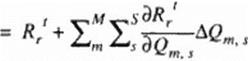
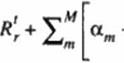
Nonce that the total number of equations in the system is the same as the total number of unknown components of Q. that is. rmax r M. If we introduce convergence rate acceleration coefficients a|. os с*ц multiplying corrections respectively, then each component.

Qm s ’> * . of the future solution vector at the grid point, s. can be extrapolated as

£ (/*»)*■ 1

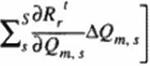This can be applied at every grid point in the domain, but it results in a huge system of imax x jmax x kmax x M unknown acceleration coefficients, a If each of the a’s is assumed to have the same value over the entire domain. D. the number of unknown a s is reduced to M. This pragmatic approach is called the global SBMR method 1311J. [312J. It requires solution of a much smaller M x M matrix. The future residual at the iteration level (t+n)+1 can. therefore, be approximated by

Subtracting (94) from (96) yields

ці’ **>♦ I

where

(102)

-4, «<‘♦*)♦ і da~

B -1*1, 5Tm

The optimum a’* arc determined such ihat Uk sum of die L-2 norm of the future resid­uals over the entire domain. D. will be minimized.

for m = With the help of (101) and (102). the system (103) becomes

In equation (101)* the R’s and a’s arc known from the preceding iteration levels. Since each am is assumed to have the same value over the entire computational domain, equation (104) gives a tractable system of M simultaneous algebraic equations for M optimum ot|. a2………………………………………………………………………………………

«М

t) (105)

For the general case of a system composed of M partial differential equations with M unknowns, the system (105) will become a full M x M symmetric matrix for M unknown opti­mum a’s.

It is plausible that for non-uniform computational grids and rapidly varying dependent variables, optimum a’s should not necessarily be the same over the whole computational domain. A modification of the SBMR method called Line Sensitivity-Based Minimal Residual (LSBMR > method was developed (311]. (312] to allow a’s to have different values from one grid line to another. The resulting system has. for example, jmax x M unknown a’s. which is quite tractable, although it is more complex to implement than the SBMR method.

The performance of the SBMR and the LSBMR methods (ЗІ I). (312} depends on how frequently these methods arc applied during the basic iteration process and on the number of iterations performed with the basic iterative algorithm that arc involved in the evaluation of the change of the solution vector. In the case of two-dimensional incompressible viscous flows without severe pressure gradient, the SBMR and LSBMR methods significantly accelerate the convergence of iterative procedure on clustered grids with the LSBMR method becoming more efficient as grids are becoming highly clustered The SBMR and the LSBMR methods tested for a two-dimensional incompressible laminar flow maintain the fast convergence for highly non- orthogonal grids and for flows w’ith closed and open flow separation The SBMR method is capable of accelerating the convergence of inviscid. low Mach number, compressible flows where the system is very stiff. An Alternating Plane Sensitivity-Based Minimal Residual (APSBMR) method (312]. a three-dimensional analogy of the LSBMR method, has been shown to successfully reduce the computational effort by 509f when solving a three-dimensional, lam­inar flow through a straight duct without flow separation.

The general formulation of these acceleration methods is applicable to any iteration scheme (explicit or implicit) as the basic iteration algorithm. Hence, it should be possible to apply these convergence acceleration methods in conjunction with the other iteration algonthms
and with other acceleration methods (preconditioning (307). multigndding (310), etc.) to explore the possibilities for a cumulative convergence acceleration effect.

In the case of optimization methods based on sensitivity analysis, live main difficulty is to make the evaluation of the derivatives less difficult and more reliable. A worthwhile effort is to research further on use of the automatic differentiation (ADIFORj based on a chain-rule for evaluating the derivatives of the functions defined by flow analysis code with respect to its input variables [313|-(317). This approach still needs to be made more computationally efficient. One obvious possibility is to utilize parallel computer architecture in the optimization process not only with the gradient search algorithms 13181, (319]. but especially with genetic evolution algorithms (320) where massively parallel approach should offer impressive reductions in com­puting time. The use of parallel computing will become unavoidable as the scope of optimiza­tion becomes multi objective (321|-(325).

An equally worthwhile effort is to further research the "one shot" method that carefully combines the adjoint operator approach and the mullignd method (326]. This algorithm opti­mizes the control variables on coarse grids, thus eliminating costly repetitive flow analysis on fine grids during each optimization cycle The entire shape optimization should be ideally accomplished in one application of the full multigrid flow solver 1326).

Finally, it should be pointed out that although the exploratory efforts in applications of neural networks (327). (328) and virtual reality arc still computationally inefficient, their time is coming inevitably as wc attempt to optimize the complete real aircraft systems. Recent pioneer­ing efforts (3291 in coupling wind tunnel experimental measurements and a muluobjective hybrid genetic optimization algorithm indicate that the decades old dream of effectively and harmoniously utilizing both resources is soon to become a reality.