Our heavyweight helicopter equal in the world does not have
In Rostov started production of the most load-lifting rotary-wing car The Russian holding «Helicopt[...]

Everything about aircrafts and helicopters. News and events in aviation worldwide. Civil, transportation, military helicopters and airplanes.

Everything about aircrafts and helicopters. News and events in aviation worldwide. Civil, transportation, military helicopters and airplanes.

Everything about aircrafts and helicopters. News and events in aviation worldwide. Civil, transportation, military helicopters and airplanes.

Everything about aircrafts and helicopters. News and events in aviation worldwide. Civil, transportation, military helicopters and airplanes.


In performing numerical simulation of practical problems, sometimes one is forced to use a relatively small computation domain. This may be because of computer memory constraint or the need to reduce computation time. In these cases, flow into or out of the scaled down computational domain could be due to the influence of sources or forces located outside as well as inside the computational domain.
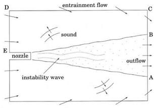
Figure 9.2. Computational domain for numerical simulation of jet noise generation.
 To maintain an accurate simulation, it is necessary to develop special boundary conditions to account for these effects on the flow inside the computational domain.
As an example, consider simulating a jet flow and noise radiation as shown in Figure 9.2. For practical reasons, the size of the computational domain is typically thirty to forty jet diameters in the axial direction and twenty to thirty diameters in the radial direction or smaller. These dimensions are somewhat smaller than those of a typical anechoic chamber used in physical experiments. Because of the proximity of the computation boundary to the jet flow, the boundary conditions along boundary BCDE are burdened with multiple tasks. Obviously, the boundary conditions must be transparent to the outgoing acoustic waves radiating from the jet. In addition, the boundary conditions must impose the ambient conditions on the numerical simulation. In other words, they specify the static conditions far away from the jet. Furthermore, the jet entrains a large volume of ambient gas. The entrainment flow velocity at the computational boundary, although small, is not entirely negligible. For high-quality numerical simulation, the boundary condition must, therefore, allow an as yet unknown entrainment flow to enter or leave the computational domain smoothly as well.
In Section 6.5, a set of radiation boundary conditions for nonuniform mean flow is provided. Let p, U, v, and p be the weakly nonuniform mean flow at the boundary region of the computational domain. The radiation boundary condition in three-dimensional cylindrical coordinates may be written as
![]() (9.4)
(9.4)
where (r, ф, x) are the cylindrical coordinates, в is the polar angle in spherical coordinates with the x-axis (flow direction of the jet) as the polar axis, and (u, v, w) are the velocity components in the axial (x), radial (r), and azimuthal (ф) directions.
V(в, r) = Ucos в + v sin в + [a2 – (v cos в — Usin в)2]/2, and a is the speed of sound.
Figure 9.3. Determination of the entrainment flow of a jet by the point-sink approximation.
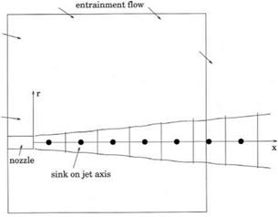
Note that the entrainment flow at the boundary region of the computation domain would be influenced by the jet flow outside the computational domain as well as inside. To develop an asymptotic entrainment flow solution, a simple way is to divide the jet into many slices as shown in Figure 9.3. The energetic portion of a jet may extend, depending on jet Mach number, beyond the computation domain to about forty diameters downstream. The mass fluxes across the boundaries of each jet slice may be found from available empirical jet flow data. The difference in mass fluxes at the two ends of each slice of the jet gives the amount of entrainment flow for the particular slice. This entrainment may be simulated by a point sink located at the center of the slice. The asymptotic solutions for a point sink located on the x-axis at xs in a compressible fluid is given by (a subscript “e” is used to indicate entrainment flow)
where pm, am, and y are the ambient gas density, the sound speed, and the ratio of specific heats, and Q is the strength of the sink. It has dimensions of pmamD2 where D is the jet diameter. On replacing (p, u, v, p) of Eq. (9.4) by (pe, ue, ve, pe) of Eq. (9.5) and upon summing over the contributions from all the sinks to approximately 60D downstream from the nozzle exit, the desired radiation-entrainment flow boundary conditions are obtained.
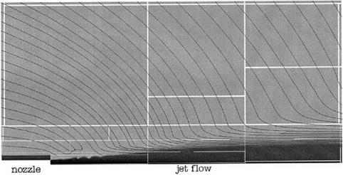
Figure 9.4 shows the entrainment flow streamlines of a Mach 1.13 cold jet from a convergent nozzle computed using the radiation-entrainment flow boundary condition. It is worthwhile to point out that along the right-hand boundary BC, the mean
|
Figure 9.4 Computed streamlines of the entrainment flow around a supersonic screeching jet at Mach 1.13. White lines separate different computation blocks. |
flow actually flows out of the computational domain, exactly as observed in free jet experiments. The streamline pattern would be vastly different had the entrainment flow outside the computational domain not been included in the sink flow computation. If the sinks outside the computational domain are excluded in forming (p, U, v, p) then a recirculation pattern would emerge. This, however, is inconsistent with experimental observations.
In this jet flow and noise radiation example, the jet may be subsonic and supersonic. For a subsonic jet, the nozzle exit pressure is nearly equal to ambient pressure, but for supersonic jets operating at off-design conditions, the pressure at the nozzle exit is quite different from that at ambient pressure. In this case, it is vital that the boundary conditions can communicate to the computation what the ambient pressure, density, and temperature are. Radiation boundary conditions (9.4) allow the specification of an ambient condition. The time-independent solution of (9.4) is и = U, v = v, p = p, andp = p. Many other radiation boundary conditions, designed with different objectives in mind, do not allow the imposition of an independent ambient condition. If these boundary conditions are used for computing an imperfectly expanded jet, the jet will not expand properly in the simulation.