RANS Computation: the k – e Model

For engineering applications, sometimes it is sufficient to compute the mean velocity profile of a turbulent flow. For this purpose, it has been recognized that the effect of turbulence on the mean flow may be adequately accounted for by including a turbulence-induced stress field. This is the Boussinesq approach. In this approach, the stress field is modeled by relating it to the strain rate field of the mean flow similar to that of laminar flow. This turbulence modeling approach is simple and relatively easy to implement on a computer. For this reason, it has become a wildly popular tool for solving practical problems for which only the mean flow is required.

Turbulence modeling is by now a well-established subject. An in-depth discus­sion of turbulence modeling is beyond the scope of this book. The objective here is to provide an introductory presentation of the subject. There are two most popular two-equation turbulence models. They are the к – є model and the к – ю model (Wilcox, 1998). A one-equation model by Spalart and Allmaras (1994) is also often used. It is now known that the к – є model works well for free shear turbulent flows, while the к – ю model works well for turbulent fluid layers adjacent to a solid surface. Motivated by this observation, Mentor (1994a, 1994b, 1997) has developed combined models, which is a clever way of blending the two models together for

computing boundary layer type flows. In this book, only the к – є model is discussed and only to a limited extent.

The к – є turbulence model has been widely used in association with the RANS equations for turbulent mean flow calculations. However, it has been recognized that the applicability of the original к – є model is quite limited. This is because the model contains only a bare minimum of turbulence physics. Also, it is because the unknown constants of the original model were calibrated primarily by using low Mach number boundary layer and two-dimensional mixing layer flow data [see Hanjalic and Launder (1972), Launder and Spalding (1974), Launder and Reece (1975) and Hanjalic and Launder (1976)].

The useful range of the к – є model has since been extended. The extensions were carried out in two ways. First, a number of correction terms, intended to incor­porate additional turbulence physics in the model, were proposed. Notable model corrections are the Pope (1978) correction developed for use in three-dimensional jets, the Sarkar and Lakshmanan (1991) correction developed for use when the convective Mach number is not too small, and the Tam and Ganesan (2003) correc­tion developed for nonuniform high-temperature flows. Second, for application to a specific class of turbulent flows, the empirical constants of the original model were recalibrated using a large set of more appropriate data. The motivation for recali­bration is the recognition that these constants are not really universal. The model would have a much better chance to be successful if it were applied to a restricted class of flows with similar turbulent mixing characteristics. For each class of flows, a new but more suitable set of constants is used. For instance, for calculating jet and free shear layer mean flows, Thies and Tam (1996) recalibrated the unknown model constants by using a large set of jet flow data covering a wide range of Mach numbers. Their computed jet mean flow velocity profiles for ambient temperature jets were found to be in excellent agreement with experimental measurements. More recently, applications of the recalibrated model to jets in simulated forward flight, coaxial jets, and jets with inverted velocity profile (see Tam, Pastouchenko, and Auriault (2001)) have been carried out with equal success.

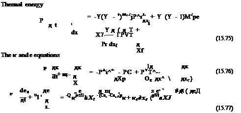
The RANS equations including the к – є model in dimensionless form may be written as follows. Here, for jet flows, dimensionless variables with D, Uj, pj, Tj (nozzle exit diameter, jet velocity, density, and temperature) as the length, velocity, density, and temperature scales will be used. Time, pressure, and the turbulence quantities к and є will be nondimensionalized by D/Uj, PjU2j, u2, and uj/D, respec­tively. Turbulent stresses ті;. and eddy viscosity uT will be nondimensionalized by u2 and Uj /D. In Cartesian tensor notation, the Favre-averaged equations of motion including the к – є model, as well as the Pope, Sarkar, and Tam and Ganesan cor­rection terms (in dimensionless form) are as follows:

Continuity

(15.73)

Momentum

dp – d(p Тц)

dxi dxe

where y is the ratio of specific heats, Pr is the Prandtl number, and Mj is the jet Mach number. There are nine empirical constants in the preceding system. The values recommended by Thies and Tam (1996) and Tam and Ganesan (2004) for jet and similar type of flows are as follows:

C, = 0.0874, Ce1 = 1.40, Ce2 = 2.02, Ce3 = 0.822, Cp = 0.035,

YoT = Pr = 0.422, ok = 0.324, ae = 0.377, a = 0.518

The RANS equations and the к – e model were originally developed with the intention for computing the mean velocity profiles of turbulent flows. The question arises as to whether they can be used for computing unsteady flow and noise. For unsteady flow application, the set of equations is, generally, referred to as Unsteady Reynolds Averaged Navier-Stokes (URANS). Clearly, there are limitations to such

usage. However, the system of URANS equations is relatively simple to use. It requires computational resources that are not too demanding. At present, there is no consensus as to whether it is appropriate to use such a formulation for noise prediction. Evidently, for certain types of problems, its use can be justified, whereas for other types it is not. One must decide based largely on the physics of the problem.