Category A PRACTICAL. APPROACH TO. ROBUSTNESS. ANALYSIS

Conclusion

[1]As mentioned in chapter 2, this assumption can not be done in the case of future large dimension transport aircrafts.

since the problem of computing the exact value of ц is known to be NP hard.

[2] We can now come back to the original problem, which is to transform the uncertain closed loop of Figure 1.3 into the standard interconnection structure M(s) – A(s) of Figure 1.1. This is very easy, since M(s) is simply the transfer matrix, which is seen by the model perturbation Д(я) on Figure 1.3 (i. e. the transfer between w and z).

[3] More generally, if the closed loop contains m neglected dynamics A{ (s), it can be transformed into the standard interconnection structure M(s) — A(s) with:

A(s) = diag(Ai(s),…, Am(s)) (1.10)

The unit ball ДДД is introduced in the space of transfer matricesA(s): BA(s) – {Д00 = diag(Ai(s),.. .,Am(s)) ||A(s)||oo < 1} (1-П)

‘The parametric uncertainties 5j may enter in practice in numerous other ways the (state – space or input/output) plant model. See chapter 3 for more details.

[4]the degree a of stability of a state-space matrix A is defined as a = max; Re(Xi(A)), where W) is an eigenvalue of A.

[5]An other reason for handling repeated complex scalars is historical: during the Eighties, the real repeated scalars were often assumed to be complex, because the real nature of parametric uncertainties could not be taken into account by existing computational algorithms.

[6] The usefulness of /X bounds is now explained. For the sake of clar­ity, we restrict our attention to the case of a real model perturbation

[7]For historical reasons, the special case of a complex model perturbation can be included in the general case of a mixed model perturbation.

[8]The LFT of equation (7.3) is assumed to be well-posed despite the uncertainties in Д2.

[9]See also chapter 11 (subsection 1.1) for the definition of a one-sided uncertainty.

[10] Condition (10.28) in the above Proposition can be simply rewritten as a {Hu) < 1, which is equivalent to the condition ст(Мц) < 1 in Lemma 4..1.

• Let Д2 = 6u>Im. The assumption к < І/^дЛМгг) in Lemma 4..1 means that the LFT Fi(H(u}o),8ujIm) (or equivalentlyi?;(fl’,8u>Im) since #22 = H22) is well-posed: see the discussion in subsection 4.2.

• Lemma 4..1 can thus be applied. Equation det{I — бшН) = Ocan be rewritten as det(l/8u>I – H) = 0, which means that the 8ш’s satisfying this last equation are the inverses of the eigenvalues of TL.

[11]It could also be interesting to consider the alternative problem, which is to compute the maximal size of the model uncertainties, for which a robust delay margin is guaranteed.

[12] The robust delay margin is to be computed, i. e. the minimal value of the MIMO delay margin when the model perturbation A belongs to its unit ball (see the end of subsection 1.2). With reference to equation (11.7), this reduces to the computation at each frequency of Ді is indeed to be maintained inside its unit ball J5Ai, while the rcj’s in A2 are to be expanded in [0, к]. Note indeed that xt є [0, k is equivalent to ті Є [0,r] in the relation:

[13] Alternatively, the singularity ofthe matrix I~P2i(jiL)A2 means that the LFT Р,(Р0’«).Да) is not well-posed.

[14] Some results in (Katebi and Zhang, 1995) are recalled here. See this reference for details. We come back to the problem of subsection 2.1 (see also Figure 12.1). The issue is to take into account the super har-

[15]The/i lower bound by (Dailey, 1990) is used in this section. Because the real model un­certainty Д2 ally contains 3 parametric uncertainties, this ^ lower bound coincides with the exact value of ц.

The general aim of this book was to emphasize the usefulness of the p approach for practical robustness analysis problems. The p and skewed p tools were first introduced. Their efficiency was then illustrated through realistic examples, namely a flight control system for a civil aircraft, a missile autopilot and a telescope mock-up.

Consider an LTI plant subject to LTI model uncertainties. These ones can be divided into two main categories, namely the parametric uncertainties (which more generally represent the uncertainties in the plant dynamics inside the control bandwidth) and the neglected dynam­ics (which represent the uncertainties outside the control bandwidth). Assuming that a controller was synthesized with the nominal model of the plant, the issue is to study the effect of these uncertainties on the closed loop stability and performance properties.

It was shown in chapters 1 and 7 that the s. s.v. P and its skewed ver­sion z’ provide a general framework for treating most of the robust sta­bility and performance problems. The only requirement is to transform the closed loop with all its uncertainties into a standard interconnec­tion structure: in this context, the main problem is to account for the parametric uncertainties, which may enter the open loop plant model in numerous ways. It is most generally possible to transform the plant model with its parametric uncertainties into a standard form, namely an LFT (part 2).

In chapter 7, it was emphasized that large classes of p problems, such as robust performance analysis, are skewed p problems, i. e. a single ap­plication of the /z tool provides in these cases just a robustness test. A recursive application of the /z tool is thus necessary to compute the ro­bustness margin. Because of the practical usefulness of these skewed p problems, a much more efficient solution is to directly compute a bound

of the skewed s. s.v. u.

Various methods were thus presented in chapter 8 for computing bounds of the skewed s. s.v. v, while chapter 5 described methods for comput­ing bounds of the classical 5.5. v. p. These techniques can be classified according to 3 different criteria:

■ nature of the result: upper and lower bounds of the (skewed) s. s.v. are generally computed instead of the exact value, the main reason being the computational requirement.

■ nature of the model uncertainties: when the problem only contains parametric uncertainties, the associated model perturbation is said to be real. On the contrary, this model perturbation is complex if there are only neglected dynamics. In the general case of parametric uncertainties and neglected dynamics, the associated model perturb­ation is said to be mixed. A great deal of work has been devoted to the computation of (a bound of) the real s. s.v.. On the other hand, methods for computing bounds of the complex s. s.v. have been lately extended to the mixed case.

■ Computational requirement: the algorithms are either polynomial time, or exponential time, i. e. the computational burden is a polynomial or exponential function of the size of the problem.

All methods in chapters 5 and 8 were evaluated on the aeronautical examples, and it was illustrated that the robustness margin can be com­puted with a satisfactory accuracy, even for large dimension problems: in the context of a problem involving a large number of uncertainties, our approach was to compute lower and upper bounds of this margin us­ing polynomial time algorithms. Even if the gap between these bounds can not be guaranteed a priori, it appears reasonable in our realistic ex­amples.

As a final point, the usefulness of the p and skewed p tools was briefly illustrated in part 5 for three non standard problems:

■ A computationally efficient method was proposed, for directly com­puting an interval of the maximal s. s.v. over a frequency interval. Good results were obtained in the examples, and an accurate estim­ate of the robustness margin was computed.

■ The issue was then to analyze the robustness properties of a closed loop in the face of parametric uncertainties, neglected dynamics and uncertain time delays. This is not a classical problem, since delays do not correspond to classical LTI finite-dimensional transfer functions.

It is nevertheless possible to parameterize the frequency response of these delays in order to reduce the problem to a standard // problem.

■ Let a linear closed loop system with additional separable nonlinearit­ies (e. g. saturations). Classical methods exist for detecting the pres­ence or the absence of limit-cycles in this closed loop. The /л approach enables to extend these classical methods to the case of parametric uncertainties entering the linear part of the closed loop.

AN APPLICATION

AN APPLICATION

The necessary condition of oscillation is used to synthesize a controller, which modifies the characteristics (magnitude and frequency) of a limit – cycle. This is an interesting engineering problem, since a limit-cycle is not necessarily a trouble in a nonlinear closed loop: a high frequency limit-cycle can linearize in an approximate way the nonlinear closed loop. Within the fj, framework, the following example illustrates that a troublesome limit-cycle (with a large magnitude and a low frequency) can be moved into a suitable limit-cycle (with a smaller magnitude and a higher frequency). For the sake of clarity, this example is chosen will­ingly simple: it is nevertheless straightforward to extend the method to the more general case of a MIMO nonlinearity, with a more complex parameterization of the controller.

Let the closed loop system of Figure 12.9, where G(s) is the plant model and K(s) the controller:

Подпись:1

Подпись: (12.37) 10 rad/s ands2 + 1.4s + 1
К

агв2 + ais + 1

AN APPLICATION

with К = 20, а,2 = 1/ta2 = 0.01, a = 2£/u; = 0.14, w £ = 0.7.

A saturation is present at the plant input (see equation (12.26)). A limit-cycle is obtained, whose predicted characteristics are a magnitude X = 2.46 and a frequency ш — 3.16 rad/s (using the method of subsec­tion 2.1). The characteristics obtained in simulation are X = 2.56 and и = 3.08 rad/s: these values are thus very close to the predicted ones, which means that the first harmonic assumption is valid. The limit-cycle is moreover stable.

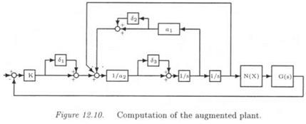
This limit-cycle is to be moved by retuning the controller K(s). The tuning parameters are K, ai and a 2 (more precisely 1 / аг). The aug­mented plant of Figure 12.3 is simply obtained by directly introducing "uncertainties" Si into the physical model of K(s) (see Figure 12.10 – N(X) is the SIDF of the saturation). The real model perturbation Д2 is Д2 = diag(6i, 62,63).

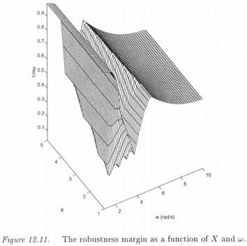
The quantity l/max(^a(Fu(P(jw), AT(Jf, w))),^2(P220’w))) is presen­ted as a function ofX and ш on Figure 12.11 (see Corollary 3..4) [15]. Re­member that there is a limit-cycle in the nominal closed loop system, at

AN APPLICATION

X = 2.46 and w = 3.16 rad/s. As a consequence, r(X, ш) = Oat this point, and r(X, u) increases around this critical point.

The limit-cycle is to be moved at X = 1.2 and ш = 6.2 rad/s (i. e. the frequency of the limit-cycle is roughly multiplied by a factor 2, while the magnitude is divided by the same factor). А ц lower bound is computed for fj, A2(Fu(P(ju}),N(X))) at this new point (X, w), namely 1.22. An associated model perturbation A?; is provided as:

<5i = 0.6906 S2 = -0.7893 S3 = 0.8203 (12.38)

This model perturbation is applied to K(s), which becomes:

Подпись: (12.39)33.81

0.0055s2 + 0.0295s + 1

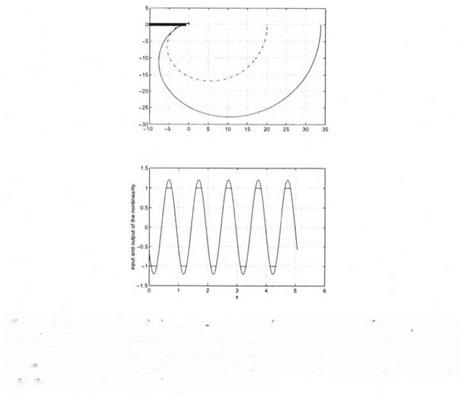
Here again, a stable limit-cycle is obtained in simulation, with A = 1.207 and ш = 6.282 rad/s (see Figure 12.12).

Подпись: Figure 12.12. Подпись: The new limit-cycle Подпись: the top Figure represents A (jui)G(jui) and

AN APPLICATIONRemark: remember first that r(X, ui) represents the minimal size of the model perturbation Д 2 , for which a limit-cycle is obtained at [Х, ш) (see definition 3..2). In the context of the above design problem, a limit-cycle is obtained for the nominal value of the controller, and this controller is retuned in order to move the limit-cycle at a point (X, u>): it is thus interesting to use the minimal size model perturbation associated to r(X, w). Indeed, the corresponding controller can be considered as the controller, which is the closest to the nominal one, and which moves the limit-cycle at (X, ci).
— 1 /N(X) in the Nyquist plane, while the lower subfigure represents the input and output of the nonlinearity (when the limit-cycle is obtained) – the dashed plot on the top Figure represents K(ju)G{jui) for the initial value of the controller, whereas the solid line represents K(ju>)G(jui) for its final value.

4. CONCLUSION

The general aim of this chapter was to check the existence or the ab­sence of limit-cycles in a closed loop subject to parametric uncertainties. The aim was more precisely to show that this nonlinear problem can be solved with existing tools of linear robustness analysis (i. e. analysis of

the robustness properties of an LTI closed loop system, subject to LTI

model uncertainties):

■ Computation of the frequency response of a parametrically uncertain transfer function (Kheel and Bhattacharyya, 1994).

■ Use of the LFT framework to transform the original problem into an equivalent standard interconnection structure.

■ Computation of upper and lower bounds of the (skewed) structured singular value.

This page intentionally left blank

A SKEWED ц PROBLEM

• With reference to chapter 8 (subsection 2.1), the computation of r(W, ca) at a point (X, ca) is a skewed ц problem, which involves a mixed uncer­tainty A = diag{Ді, Д2) (Ai is here a fictitious full complex block). It is consequently possible to use the first mixed skewed ц bound of chapter 8 (section 1.). Otherwise, the special structure of the problem can be accounted for, and this specific skewed /u problem can be transformed into an augmented p problem: see chapter 8 (section 2.). This solution is easier to implement, since standard p tools are directly available in Matlab Toolboxes (such as the ц Analysis and Synthesis Toolbox or the LMI Control Toolbox).

• A sufficient condition of non-oscillation is used in this section. A skewed Ц upper bound is thus more attractive than a skewed ц lower bound, whose interest is only to measure the conservatism of the upper bound. Indeed, even if a model perturbation A* is obtained, which does not satisfy the sufficient condition of non oscillation, this does not mean that a limit-cycle is obtained when applying A* to the closed loop. On the contrary, the ц upper bound gives a maximal size of the parametric uncertainties, for which the absence of limit-cycle is guaranteed.

EXTENSION TO THE CASE OF PARAMETRIC UNCERTAINTIES

• As a preliminary, it is straightforward to extend the graphical method

in the previous subsection (see also Figure 12.6) to the case of a transfer function G(s,6), which depends on some parametric uncertainties Sp see section 2.2.

Подпись: Q(X,u>)

Figure 12.8. Small gain test for checking the absence of limit-cycles – extension to

parametric uncertainties.

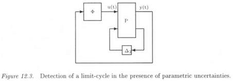
• The general case of a MIMO nonlinearity is considered. As in section 3.1, parametric uncertainties are introduced in the closed loop of Fig­ure 12.1 byrewriting C7(s,£)as an LFT F)(P(s), Д2), where Дгів areal model perturbation (see Figure 12.3). Replacing then Ф by its frequency response N(X, ш) + А, Figure 12.3 is transformed into figures 12.8.a and 12.8.b. The sufficient condition of non oscillation is:

m(Q(X, u>), Д2)) < -7^-r (12.35)

0!(A, U>)

The robustness margin is the maximal size of parametric uncer­

tainties, for which the sufficient condition above is satisfied.

DEFINITION 4..1

r(X, w) = min (k ЭД2 e kD-2 s. t. a(F,(Q(X, u), Д2)) > * – Л (12.S6)

J

r(X, w) = 0 if the nominal closed loop (obtained with A2 = 0) does not satisfy equation (12.34).

Remark: in the case of a diagonal MIMO nonlinearity, diagonal scaling matrices V can be introduced in the small gain test, in order to reduce the conservatism of the sufficient condition of non oscillation (i. e. to con­sider a(T>Fi(Q(X, u>),A2)V~1) instead of a(Fi(Q(X, to), Д2)) in defini­tion 4..1).

A SECOND ц BASED METHOD

The sufficient condition of non oscillation is introduced in the first subsection. The method is extended to the case of parametric uncertain­ties in the second subsection. The third subsection shows that a skewed H problem with a special structure is to be solved. The problem of using (skewed) /г bounds is discussed in the last subsection.

3.2 A SUFFICIENT CONDITION OF NON OSCILLATION

A SECOND ц BASED METHOD

monic part e(£) of the signal u(t), at the output of the nonlinearity Ф. To this aim, the frequency response of the nonlinearity is rewritten as N(X, uj) + Д, where Д represents the error induced by the SIDF approx­imation.

• In the case of a SISO nonlinearity, Д is known by the relation:

A SECOND ц BASED METHOD

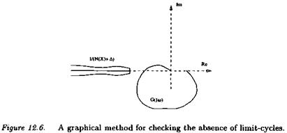
where a( X, a( is a function of X and ш. With respect to Figure 12.1, a sufficient condition of non oscillation is then that the inverse of the frequency response X( X, a) X Д of the nonlinear element does not inter­sect the frequency response of the linear part G(s) of the closed loop. As in section 2.1, when N(X, w) and a{X, u>) do not depend on frequency u>, Figure 12.6 suggests a graphical method for checking the absence of limit-cycles.

A SECOND ц BASED METHOD

• In the case of a MIMO nonlinearity, Д is known by the relation:

a(A)<a(X, u) (12.32)

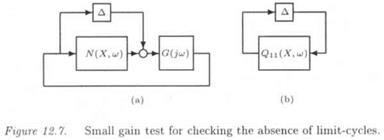
Figure 12.1 is transformed into Figure 12.7. a, by replacing the nonlinear­ity Ф by its frequency response N(X, u>) + A. Figure 12.7.a is then trans­formed into Figure 12.7.b, where Qn(X, w) is the transfer seen by Д in Figure 12.7.a Applying finally the small gain theorem to Figure 12.7.b, a sufficient condition of non oscillation is obtained as:

A SECOND ц BASED METHOD

where Д satisfies equation (12.32). The sufficient condition of non oscil­lation thus becomes:

A SECOND ц BASED METHOD

THE USE OF д BOUNDS

A necessary condition of oscillation is used in the above method. With reference to the end of section 3.1, two different cases are to be considered:

■ If no limit-cycle is obtained for the nominal closed loop system, the aim is to find the minimal amount of parametric uncertainties, for which a limit-cycle is obtained. It is interesting in this context to

compute both upper and lower bounds, since the flower bound (resp. the / upper bound) gives a size of the parametric uncertainties, for which the necessary condition of oscillation is satisfied (resp. not satisfied). The ц lower bound moreover gives a model perturbation Д[14], for which the necessary condition of oscillation is satisfied. It is then interesting to apply Д* to the closed loop, in order to check whether the first harmonic approximation is valid and whether the corresponding limit-cycle is stable or unstable (see section 5.).

■ If a limit-cycle is already obtained for the nominal closed loop sys­tem, the idea is rather to visualize the movement of this limit-cycle (i. e. the variation of its amplitude and frequency) as a function of the parametric uncertainties. In this new context, it is more interesting to obtain a model perturbation Д*, which satisfies indeed the necessary condition of oscillation. A /x lower bound is thus more interesting than a Ц upper bound.

AN EXTENSION

In the above method, /ад2(Fu(P(juj), N(X, u))) is to be computed at each point (X, u>) of a gridding. The robustness margin r(X, u>) is then visualized as a function ofX and ы on a 3D plot (see section 5.). Nev­ertheless, a peak value of y&2(Fu(P(juj),N(X, uj))) may be missed with such a gridding (i. e. when this peak value lies between two points of the gridding), and the robustness properties of the closed loop would be overevaluated.

A simple method is proposed here for avoiding a gridding of the mag­nitude X, by treating this magnitude (more precisely the SIDF N(X, u>)) as an additional (fictitious) uncertainty. Frequency ш is fixed. An aug­mented skewed Ц problem is obtained. Even if the method is not applic­able to all kinds of nonlinearities, it can be applied to a large class of usual (especially memoryless) ones.

• The aim of this subsection is to compute the robustness margin r(o>)

r(ui) = min_ r(X, w) (12.24)

хє[£, X]

Lemma 3..5 provides an alternative definition of r(u>). The proof is trivial when using Proposition 3..3.

LEMMA 3..5 If:

l/r{u) < l/HA2(P22(ju)) _

2/ det(I – Pn(ju})N(X, u})) ф 0 for all X Є [X, X]

then:

Подпись: (12.25)-ГТ = max_ /j, A2{Fu{P(ju>),N{X, u>))) r(u) xe[x, x]
• Consider first a classical nonlinearity, namely a saturation у = Ф(ж)

у = x if x < 1 = +1 if X > 1

= -1 if X < -1 (12.26)

AN EXTENSION

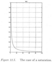
The associated SIDF N(X), which does not depend on frequency u> and which is a real scalar, can be computed as (see also Figure 12.5):

With respect to Figure 12.5 and equation (12.27), it is obvious that X € [0, oo] leads to N{X) Є [0, 1].

AN EXTENSION

• Consider now the generic case of a memoryless SISO nonlinearity: here again, the SIDF N(X) is a real scalar which does not depend on frequency и). X Є [X, X] can thus be translated into N(X) Є [jV, N], The idea is thus to rewrite N(X) as:

N{X) = a0 + a xx (12.28)

where the oti s are chosen so that x — [ — 1 , 1 ] leads to N(X) є [N, IV].

• In the general case of a diagonal MIMO memoryless nonlinearity Ф = сІіад(Фі), the SIDF can be written as:

N(X) = Z0 + ZiA і (12.29)

where the Zi s are fixed diagonal matrices and Ді = diag(xi). X denotes now a vector of magnitudes Xu while_N(X) is a diagonal matrix. Here again, Ді Є D leads to N(X) e [N_, N], • Applying now equation (12.29) to Figure 12.3, this Figure can be trans­formed into Figure 12.4, where:

■ the fictitious real model perturbation — i contains the uncertainties Xi in the magnitude vector X, or equivalently in the SIDF N(X).

■ the real model perturbation Д2 contains the true parametric uncer­tainties.

■ Matrices Zi ’ s are incorporated in the transfer matrix P(s).

The following Proposition presents a method for computing r(u). PROPOSITION З..6 Let the interconnection structure of Figure 12.4. If:

1/г{ш) < 1/мд2(РЫ. Н)

2//W-PiiO’w)) < 1

then:

AN EXTENSION

г’д(P(jw)) is the skewed s. s.v. associated to the complex matrix P(jaj) and to the real model perturbation Д = diag{Aі, Дг)- Ді is to be main­tained inside its unit hypercube D.

Remarks:

(i) The assumptions of this Proposition are essentially extensions of the assumptions in Proposition 3..3. Note especially that the second assump­tion in Proposition 3..6 means that the necessary condition of oscillation is not satisfied by the nominal closed loop system, for frequency to and for a vector of magnitudes X є [X, X].

(ii) A frequency gridding can be avoided, by treating ю as an additional uncertainty in an augmented ц problem (see section 3. of chapter 7).

(Hi) The above method can be applied to nonlinearities, which are not necessary memoryless: The SIDF N(X, uj) may depend on w and it may take complex values. For a fixed value of u>, the key point is to be able to reparameterize N(X, u>) in an affine way as N(X, u>) = ao + оцх, so that the trajectory of N(X, w) in the complex plane is the same when imposing s Z [ — 1 , 1 ] and X Є [X, hi­proof: this Proposition is an extension ofProposition 3..3 and Lemma 3..5 The issue is to compute the maximal value ofr(X, u>) over X Є [X, X]. The fictitious parametric uncertainties Xi associated to N(X) must con­sequently remain inside the unit hypercube D, while the true parametric uncertainties in Д2 are to be expanded, until the necessary condition of oscillation in equation (12.14) is satisfied.

A GENERALIZED CONDITION OF OSCILLATION

Nonlinearity Ф is replaced in Figure 12.3 by its SIDF N(X, u). It is then straightforward to transform Figure 12.3 into Figure 12.4.a, with Ді replaced by N(X, w). Assume a fixed value for matrix Д2 (and thus for the associated vector <5 of parametric uncertainties) in Figure 12.3.

In the case of a SISO nonlinearity Ф, the necessary condition for the existence of a limit-cycle is:

Подпись: (12.13)l-Fi(P(ju>),A2)N(X, u) =0

In the general case of a MIMO nonlinearity, the necessary condition becomes (Gray and Nakhla, 1981):

Подпись: (12.14)det(I – Fl(P(juJ),A2)N(X, u)) = 0

X and to are fixed in this subsection, so that N(X, ш) is a constant mat­rix. As a consequence, the matrix Fu(P(jw),N(X, u))) (i. e. the transfer matrix at frequency o>, seen by the real model perturbation Д 2 in figure 12.4.a) can be computed a priori.

Proposition 3..3 introduces a method for computing the robustness margin r{X, ut), which measures the size of the smallest parametric un­certainty Д2, for which the necessary condition of oscillation in equation (12.14) is satisfied. Remember as a preliminary that r(X, u>) is a robust­ness margin, while the s. s.v. is homogeneous to the inverse of a robustness margin.

Definition 3..2

г(Х, ш) = min(k І ЗД2 Є kD2 s. t. det(I – Fi(P{ju), A2)N(X, u)) = 0) (12.15)

with r(X, u>) = 0 if the nominal closed loop (obtained with Д2 = 0J satisfies equation (12.14). Conversely, r(X, ut) = 00 if no Д2 satisfies equation (12.14).

1 /l*A3(P22(M) )N(X, u;))f 0

PROPOSITION 3..3 If: 1/ r(X, w]

2/ d, et(I – then r(X, u) – 1 /fiA2(Fu(P(ju),N(X, u)))

Proof: Lemma 3..1 is used. let к = r(X, w) and Ді = N(X, ui). Using the first assumption of the Proposition, it can be claimed that:

Подпись: (12.16)det(I — P22{juj)A2) ф 0 УД2 Є kD2

Using then the second assumption, it is easy to see that the assumptions of Lemma 3..1 are satisfied, so that:

det(I-F,(P(jw),A2)t1)fO <t=> det(I-Fu(P(jw),Ai)A2)f0 (12.17) r(X, uj) thus coincides with l//iA2(Fu(P(ja>),lV(.X’, w))).

Remark: the second assumption in Proposition 3..3 means that the

necessary condition of oscillation is not satisfied at (X, ш) for the nom­inal closed loop system, since Fi ( P(Д) , Д2 ) = Pi p (Д ) when Д2 = 0.

Concerning the first assumption in Proposition 3..3, it is worth point­ing out that /ід2(Р22(Д)) measures the robust stability property of the transfer matrix Fi(P(s),A2) [13] (i. e. the transfer matrix between u andy in Figure 12.3). Assume indeed that P(s) is asymptotically stable. Define then the stability margin kmax as the maximal value of k, such that the transfer matrix Fi(P(s),A2) is asymptotically stable for all Д2 Є kD2. kmax can be computed as:

77— = max HA2(P22(j<j)) (12.18)

Kmax

As a final point, the following Corollary proposes to compute a lower bound of the robustness margin r(X, u>) when the first assumption in Proposition 3..3 is not satisfied.

Corollary 3..4 If – et( i – Pi—( x( x,-) ) – о, then:

r(x’“) – <іг’19> Proof:

• If/iAJ(i;,u(P(jci;))7V(-X’,w))) > мд2(Р22(7^)), the assumptions ofPro – position 3..3 are satisfied and the above Corollary reduces to this Pro­position (Inequation (12.19) becomes an equality).

• IfHA2(Fu(P(ju),N(X, u))) < fJ. A2(P22(jw)), let к < 1 /HA2(P22(ju)) and F( p F( F, f(. By definition of /гд2(Р22(.?А;)):

det(I – P22(ju)A2) ф 0 УД2 Є kD2 (12.20)

Using then the assumption of the Corollary, it is straightforward to see that the assumptions of Lemma 3..1 are here again satisfied, so that:

det{I-F,(PUu),A2)Ai)*0 <=► det(I-Fu(PU^),Al)A2)^0 (12.21)

Noting then that к < l/i/,A2(Pu(P(ju),N(X, w))), it can be claimed that:

Подпись:Подпись: (12.23)det(I – Fu(P(ju), Ді)Д2) Ф 0 УД2 Є kD2

As a consequence:

det(I – Ft(P{jш),А2)Аі) ф 0 УД2 Є kD2

The necessary condition of oscillation of equation (12.14) is not satisfied, and к is consequently a lower bound of the robustness margin r(X, w).

. A PRELIMINARY TECHNICAL RESULT

. A PRELIMINARY TECHNICAL RESULT

A technical Lemma is needed, which forms the basis of the Main Loop Theorem (see subsection 4.4 of chapter 1). Let P a complex matrix and Ді and Д2 two mixed model perturbations. The two interconnection structures of Figure 12.4 are equivalent, if Д = diag( Ді, Д2). Partition then compatibly P as:

LEMMA 3..1 If matrices I — P22A2 and I — РцДі are invertible, then:

det(I-PA) = det{I-P22A2)det{I-Fi{P, A2)Ax)

= det{I – PnAi)det{I – Fu{P, Ax)A2) (12.11)

Proof: A classical property of the determinant is used:

Подпись: det where D is invertible. {c d) = det(D)det(A ~ BD~lC) (12.12)

A FIRST /X BASED METHOD

This section and the following one consider the general case of a MIMO nonlinearity. As a preliminary, the first subsection illustrates that the general problem of detecting a limit-cycle in the presence of parametric uncertainties can be recast into an LFT framework. A technical result is then presented in the second subsection. It is proved in the third subsec­tion that the issue of detecting a limit-cycle can be made equivalent to the issue of detecting the singularity of a matrix, which depends on paramet­ric uncertainties: this problem can thus be treated in the ц framework. An extension of the method is presented in the fourth subsection. The use of Ц bounds is finally discussed in the last subsection.

3.1 AN LFT FORMULATION OF THE PROBLEM

A FIRST /X BASED METHOD

Consider the general case of a MIMO transfer matrix G(s,6), where 5 is a vector of parametric uncertainties Si. Following chapter 3, G(s,6) can be expressed as an LFT Ft(P(s), Д2),where Д 2 is a diagonal matrix:

A FIRST /X BASED METHOD

In the generalized problem of Figure 12.3 (to be compared with Fig­ure 12.1), the aim is twofold:

■ If no limit-cycle exists for the nominal closed loop system (<5j = 0), the minimal amount of parametric uncertainties is to be found, for which a limit-cycle is obtained in the closed loop system of Figure 12.3.

■ If a limit-cycle exists in the nominal closed loop system, it is inter­esting to visualize the movement of this limit-cycle (i. e. the variation

of its magnitude X and frequency ta) as a function of parametric uncertainties.