Solution of the Flow Over Slender Pointed Wings

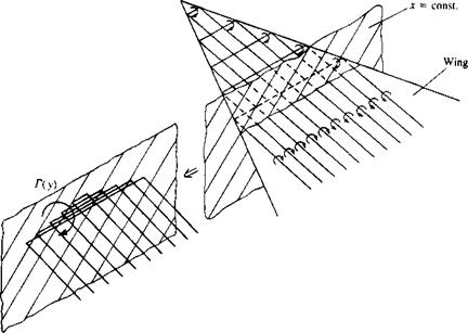
The integral equation (Eq. (8.68)) for the unknown doublet strength contains a strong singularity at у = y0 (see Appendix C for a discussion of the principal value of this integral). Recalling the results of Section 3.14 that a doublet distribution can be replaced by an equivalent vortex distribution [e. g., dii(y)/dy = — y(y)] allows us to use some of the results of thin-airfoil theory for the crossflow plane solution when the vortex distribution is used instead. The proposed vortex distribution consists of horseshoe type vortices distrib­uted continuously over the wing. This vortex model is described schematically in the right hand side of Fig. 8.17, where for the purpose of illustration,

FIGURE 8.17 Horseshoe model for the slender, thin, pointed wing.

x = const.

r(v)

-► V

2

+A 2

FIGURE 8.18 Vortex distribution in the cross – flow (x = const.) plane.

Q^o(x)

discrete horseshoe elements are used instead of the continuous distribution. At any x — const, section the trailing vortices form a two-dimensional vortex distribution of circulation per length y(y) along the strip —b(x)/2<y < b(x)/2, z = 0 as shown in Fig. 8.18. Note that in the crossflow plane, owing to left/right symmetry, the total circulation is zero, and the lift is generated by the spanwise segments of the horseshoe vortices (as shown in the left hand side of Fig. 8.17). The perturbation velocity potential for this two-dimensional crossflow (modeled by the vortex distribution shown in Fig. 8.18, and formulated in Section 3.14) at any x station is

(8.69)

Observe that the positive vorticity vector in the y-z plane points in the positive x direction, as shown in Fig. 8.18. The velocity components in the x = const, plane, due to this velocity potential, are

(8.70)

(8.71)

Because of the slender wing assumption, only the local trailing vortex distribution (parallel to the x-axis) will affect the near-field downwash. By substituting this vortex distribution-induced downwash into the wing boundary condition, Eq. (8.63) becomes

(8.72)

Comparing this form of the boundary condition with the formulation for high aspect ratio wings (Eq. (8.11)) clearly indicates that due to the slender-wing assumption the effect of the spanwise vortices was neglected. The solution for the vortex distribution, at each x station, is reduced now

to the solution of this equation for y(y) with the additional condition that

Because of the similarity between this integral equation (Eq. (8.72)) and the lifting line equation (see Eqs. (8.10) and (8.11)), a solution of similar form is proposed. Let the spanwise circulation Г(х, у), at each x section, be an elliptic distribution as in Eq. (8.21):

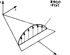
The physical meaning of this circulation is best described by observing the horseshoe vortex structure shown in Fig. 8.17 where the downwash induced by the spanwise segments of the horseshoe vortices ahead of this x station is neglected when evaluating the boundary conditions. Then if the total circulation ahead of an x — const, chordwise station is replaced by a single spanwise vortex line, as shown in the left side of Fig. 8.17, then its strength will be Г(у).

The spanwise distribution of the trailing vortices (shown in Fig. 8.18) is obtained by differentiating with respect to у (as in Eq. (8.41)):

But this integral has already been evaluated in this chapter (see Eq. (8.22)) and resulted in a constant spanwise downwash. With the use of the results of Eqs. (8.22) and (8.24) the spanwise integration yields

and Eq. (8.76) becomes

which shows that the spanwise induced downwash due to an elliptic circulation distribution is constant and independent of y. The value of Гтах is easily

evaluated now and is

To establish the relation between the velocity potential and Г consider a path of integration along the local у axis (for anr = const, section)

where the integration starts at the left leading edge of the x = const, station and the integration path is above (0+) or under (0-) the wing. Therefore, the potential jump (АФ) across the wing and the lift of the wing portion ahead of this x station (pQ<S(y)) are elliptic too:

ДФ(х = const.,у) = Ф(х, у, 0+) – Ф(дг, у, 0—) = 2Ф(х, у, 0+)

= Г(х = const., у) = Г(у) (8.80)

as shown in Fig. 8.19. Note that the local Г(у) is equivalent to the sum of all the spanwise bound vortex segments of the horseshoe elements ahead of it (see left side of Fig. 8.17) and therefore is equivalent to the lift of the wing portion ahead of this x station.

By substituting y(y) and Гтах into Eqs. (8.69-8.71), the crossflow potential and its derivatives are obtained:

This differentiation can be executed only if wing planform shape b(x) and

angle of attack a(x) are known. The spanwise velocity component is

(Note that y(y) can be obtained as a solution of Eq. (8.72) directly from Eq.

(7.18) .) Based on Eqs. (8.71-8.72) the downwash on the wing is

ЭФ

w(x, y, 0±) = — (ж, y, 0±) = -0ooOr(x) (8.84)

dZ

The aerodynamic loads will be computed with the use of the linearized Bernoulli equation (Eq. (4.53)). The pressure jump across the wing is given by

Ap =p(x, y, 0—) — p(x, y, 0+) = pQ„ —АФ (8.85)

and this pressure difference

For example, let’s assume that the wing’s angle of attack is constant a(x) = a and for this case the pressure difference becomes

a / v P П2п b(x)db(x)/dx AP(x, y) = – Q*,a-

-y

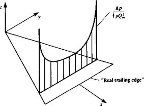
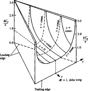
This spanwise pressure distribution is plotted in Fig. 8.20, and for a delta wing

FIGURE 8.20

Spanwise pressure difference dis­tribution of the slender wing at an x = const, plane.

with straight leading edges, the pressure difference is plotted in Fig. 8.21. It is clear from these figures that this solution has an infinite suction peak along the wing leading edges. It seems as if the trailing edges of a high aspect ratio wing (while being swept backward) were folded into the root-chord and they are not visible, and consequently the lowest Ap at each x station is at the centerchord. Also since the trailing edge is not visible, the Kutta condition is not fulfilled along the “real trailing edge,’’ which resembles the side edges of this imaginary high aspect ratio wing.

The longitudinal wing loading is obtained by an integration of the spanwise pressure difference and with the use of the result of Eq. (8.25) that

(8.88)

With this in mind,

The interesting conclusion from this equation is that if there is no change either in or(;c) or in b(x), there will be no lift due to this section. Also for a wing with linear b(x) (delta wing) and constant a the longitudinal loading is linear too.

The lift of the wing from the tip to a section x is obtained by integrating dL/dx along x :

L(x) = J ^dx = ^pQl[a(x)b(x)2] (8.90)

This means that the lift of the wing up to a given x station depends on the local ct(x), b(x) and db(x)/dx only. For the complete wing, therefore, it is a function of its maximum span b and a (at this chordwise station):

L = ^pQlab2 (8-91)

When the wing extends behind its maximum span (and the slope db(x)/dx is negative) the contribution to the lift due to this portion is excluded by this model. Therefore, by using the maximum span in Eq. (8.91) the difficulties for wings having negative db(x)/dx near the trailing edge are avoided.

The spanwise loading, at any x station, is obtained in a similar manner:

fy – PCJW – 1 – } (8.92)

which is an elliptic spanwise load distribution, as shown in Fig. 8.19. The lift up to any section x can be obtained by the integration of the spanwise loading as well:

L(x) = f ^rdy = J Р£>1[Ф)Ь(х)2] (8-93)

J-b/2 dy 4

The lift coefficient is obtained by using Eq. (8.91),

„ жЪ2 л

CL = –a = – JRa (8.94)

and the induced drag coefficient (using Eq. (8.29)) for this elliptic distribution is

со=~2СІ = сЛ (8.95)

JT t) /

If the drag force is a result of the pressure distribution only then its magnitude is expected to be CLa, but this result of Eq. (8.95) indicates that the “leading-edge suction” is reducing the drag by 1/2. This can be shown by observing the suction force acting along the leading edges, as shown schematically in Fig. 8.16, which is a result of the rapid turning of the flow at
this point. The magnitude of this force was calculated in Section 6.5.3 (

(6.52) ) and is positive along the right leading edge,

,H*)

db(x) , ті r. – b2 a *

and negative along the left leading edge (here, for simplicity, a(x) = a w&§ assumed). Since this force acts on both leading edges of the wing, no net sideforce is created; however, these forces will have a forward-pointing component of magnitude Ts:

Consequently the drag force is the pressure difference integral La minus the leading edge thrust La/2 and is equal to only one-half of La, as obtained in Eq. (8.95).

The pitching moment about the apex of the wing is

M0= [ ^xdx = ?pQl( x-^-[a(x)b(x)2]dx (8.%)

Jo dx 4 Jq dx

Again, in order to evaluate this integral, the angle of attack and span variation with x are needed. As an example, consider a flat triangular delta wing with a constant angle of attack a where the trailing edge span is bT B :

b(x) = bT, e. – c

and by substituting this into Eq. (8.96),

M0 = jPQlJ0 X~ [a^b$.E]dx = ^pQlab? t.

and the center of pressure is at the center of area

Xcp_ 4/q_ 2

c Lc 3