Integrated Equations of Motion of the Helicopter

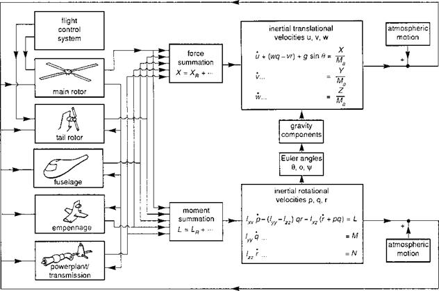
In the preceding sections the equations for the individual helicopter subsystems have been derived. A working simulation model requires the integration of the subsystems in sequential or concurrent form, depending on the processing architecture. Figure 3.39 illustrates a typical arrangement showing how the component forces and moments depend on the aircraft motion, controls and atmospheric disturbances. The general

Fig. 3.39 The integrated helicopter simulation model

where we have assumed only first-order flapping dynamics.

SCAS inputs apart, the control vector is made up of main and tail rotor cockpit controls,

u = (m, ms, mc, nor) (3.299)

Written in the explicit form of eqn 3.293, the helicopter dynamic system is described as instantaneous and non-stationary. The instantaneous property of the systemrefers to the fact that there are no hysteretic or more general hereditary effects in the formulation as derived in this chapter. In practice, of course, the rotor wake can contain strong hereditary effects, resulting in loads on the various components that are functions of past motion. These effects are usually ignored in Level 1 model formulations, but we shall return to this discussion later in Section 3.4. The non-stationary dynamic property refers to the condition that the solution depends on the instant at which the motion is intitiated through the explicit dependence on time t. One effect, included in this category, would be the dependence on the variation of the atmospheric velocities – wind gusts and turbulence. Another arises from the appearance of aerodynamic terms in eqn 3.293 which vary with rotor azimuth.

The solution of eqn 3.293 depends upon the initial conditions – usually the heli­copter trim state – and the time histories of controls and atmospheric disturbances. The trim conditions can be calculated by setting the rates of change of the state vector to zero and solving the resultant algebraic equations. However, with only four controls, only four of the flight states can be defined; the values of the remaining 17 variables from eqn 3.293 are typically computed numerically. Generally, the trim states are unique, i. e., for a given set of control positions there is only one steady-state solution of the equations of motion.

The conventional method of solving for the time variations of the simulation equations is through forward numerical integration. At each time step, the forces and moments on the various components are computed and consolidated to produce the total force and moment at the aircraft centre of mass (see Fig. 3.39). The simplest integration scheme will then derive the motion of the aircraft at the end of the next time step by assuming some particular form for the accelerations. Some integration methods smooth the response over several time steps, while others step backwards and forwards through the equations to achieve the smoothest response. These various elaborations are

required to ensure efficient convergence and sufficient accuracy and will be required when particular dynamic properties are present in the system (Ref. 3.56). In recent years, the use of inverse simulation has been gaining favour, particularly for model validation research and for comparing different aircraft flying the same manoeuvre. With inverse simulation, instead of the control positions being prescribed as functions of time, some subset of the aircraft dynamic response is defined and the controls required to fly the manoeuvre computed. The whole area of trim and response will be discussed in more detail in Chapters 4 and 5, along with the third ‘problem’ of flight dynamics – stability. In these chapters, the analysis will largely be confined to what we have described as Level 1 modelling, as set down in detail in Chapter 3. However, we have made the point on several occasions that a higher level of modelling fidelity is required for predicting flight dynamics in some areas of the flight envelope. Before we proceed to discuss modelling applications, we need to review and discuss some of the missing aeromechanics effects, beyond Level 1 modelling.