An Exercise in High-Altitude Operation

Fixed-wing aircraft operate more economically at high altitude than at low. Aircraft drag is reduced and engine (gas-turbine) efficiency is improved, leading to increases in cruising speed and specific range (distance per unit of fuel consumed). With gas-turbine-powered helicopters, the incentive to realize similar improvements is strong: there are, however, basic differences to be taken into account. On a fixed-wing aircraft, the wing area is determined principally by the stalling condition at ground level; increasing the cruise altitude improves the match between area requirements at stall and cruise. On a helicopter, the blade area is fixed by a cruise speed requirement, while low-speed flight determines the installed power needed. The helicopter rotor is unable to sustain the specified cruising speed at altitudes above the density design altitude, the limitation being that of retreating blade stall. The calculations now to be described are of a purely hypothetical nature, intended to illustrate the kind of changes that could in principle convey a high-altitude flight potential. The altitude chosen for the exercise is 3000 m (10 000 ft), this being near the limit for zero pressurization. We are indebted to R. V. Smith for the work involved.

Imperial units are used as in the previous section. The data case is that of a typical light helicopter, of all-up weight 10 000 lb and having good clean aerodynamic design, though traditional in the sense of featuring neither especially low-drag nor advanced blade design. Power requirements are calculated by the simple methods outlined earlier in the present chapter. Engine fuel flow is related to power output in a manner typical of modern gas-turbine engines. Specific range (nautical miles per pound fuel) is calculated thus:

Specific range(nm/lb) = forward speed((knots)/fuel)flow(lb/hr)

A flight envelope of the kind described in Section 7.7 is assumed: this is primarily a retreating-blade limitation in which the value of W/d (d being the relative density at altitude) decreases from 14000lb at 80 knots to 8000lb at 180 knots.

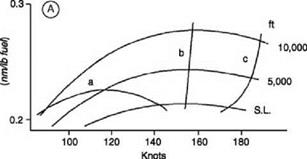
The results are presented graphically in Figures 7.9A-D.

Specific range is plotted as a function of flight speed for sea level (SL), 5000 ft and 10 000 ft altitude. Intersecting these curves are (a) the flight envelope limit, (b) the locus of best-range speeds and (c) the power limitation curve. We see that in case A, which is for the data helicopter, the flight envelope restricts the maximum specific range to 0.219 nm/lb, this

occurring at 5000 ft and low speed (only 114 knots). So far as available power is concerned, it would be possible to realize the best-range speeds up to 10000 ft and beyond.

Case B examines the effect of a substantial reduction in parasite drag. Using a less ambitious target than that envisaged in Section 7.9, a parasite drag two-thirds that of the data aircraft is assumed. At best-range speed a large increase in specific range at all altitudes is possible but, as before, the restriction imposed by the flight envelope is severe, allowing an increase to only

0. 231 nm/lb, again at approximately 5000 ft and low speed (120 knots). It is clear that the full benefit of drag reduction cannot be realized without a considerable increase in rotor thrust capability. A comparison of cruising speeds emphasizes the deficiency: without the flight- envelope limitation the best-range speeds would be usable, that is at all heights a little above 150 knots for the data aircraft and 20 knots higher for the low-drag version.

The increase in thrust capability required by the low-drag aircraft to raise the flight envelope limit to the level of best-range speed at 10000 ft is approximately 70%. Case C shows the performance of the low-drag aircraft supposing the increase to be obtained from the same percentage increase in blade area. Penalties of weight increase and profile power increase are allowed for, assumed to be in proportion to the area change. The best-range speed is now attainable up to over 9000 ft, while at 10 000 ft the specific range is virtually the same as at best – range speed, that is 0.267 nm/lb at 170 knots; this represents a 22% increase in specific range over the data aircraft, attained at 60 knots higher cruising speed.

For a final comparison, case D shows the effect of obtaining the required thrust increase by combination of a much smaller increase in blade area (24.5%) with conversion to an advanced rotor design, using an optimum distribution of cambered blade sections and the Westland advanced tip. The penalties in weight and profile power are thereby reduced considerably. The result is a further increase in specific range, to 0.293 nm/lb or 34% above that of the data aircraft, attained at the same cruising speed as in case C.

The changes are seen to further advantage by calculating also the maximum range achievable. This has been done in alternative ways, assuming that the weightpenalty reduces (1) the fuel load or (2) the payload. On the first supposition, the weight penalty of case C results in a range reduction but with case D the gain more than compensates for the smaller weight penalty.

The characteristics of the various configurations are summarized in Table 7.3.