Category A PRACTICAL. APPROACH TO. ROBUSTNESS. ANALYSIS

Let Д = diад( Д 1 , Д s ) , where the Д s ’ s are most generally mixed struc­tured model perturbations. Without loss of generality, the aim is to ana­lyze the sensitivity of the s. s.v. ц{М) with respect to the first model perturbation Дх. Let the complex matrix M be partitioned as in equa­tion (1.39), so that Mn corresponds to Ді and M22to Д2.

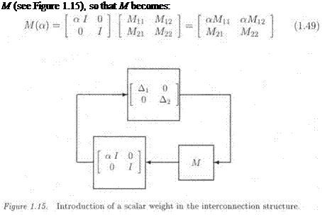
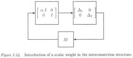
In the same way as in subsection 4.2, the model perturbation Дх is weighted by a scalar a, i. e. the model perturbation inside the intercon­nection structure becomes (see Figure 1.14):

in Figure 1.14 is transfered from Д to

Note that the weighting scalar a can be introduced in three different ways in the interconnection structure. The first one is equation (1.48). The second one is:

and the associated value of M(a) is:

Even if these 3 solutions are equivalent, the third one is often chosen for numerical reasons (Braatz and Morari, 1991). The д sensitivity with respect to Ai is defined as:

It is easily proved that д(М(а)) is a non decreasing function of a, so that <5д is necessarily non negative. Moreover, it can be proved that the — sensitivities are well-defined and equal to the corresponding full derivatives, almost everywhere on any interval of variation of a (Braatz and Morari, 1991).

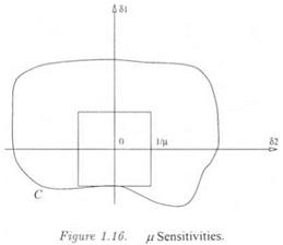
Indeed, ё ц can be interpreted as the derivative of /rwith respect to a (with the restrictions above). As a consequence, the higher the value of 6fi, the more critical the model perturbation Ді in the value of д. Consider as an illustration the case where — = 0 : this means that Ai has no influence on the value of д. Figure 1.16 illustrates this point. Let A = diag(Si,62), where the Si’s are real scalars. Figure 1.16 represents the space of the Si’s. Each point of the curve C corresponds to a value of the 0 : s, for which the matrix 0 — M A is singular. Conversely, all points strictly inside the domain, whose border is C, correspond to values of the Si’s, for which the matrix 1-М A is nonsingular. In an obvious way, the zero point (which corresponds to <5i = 0 and 82 = 0) belongs to this domain of nonsingularity.

1/д represents the size of the largest square in the space of the Si’s, which is centered on the zero point and inside which the matrix I — MA is guaranteed to be nonsingular. In Figure 1.16, the д sensitivity with respect to S2 is strictly positive, whereas the /x sensitivity with respect to S і is zero.

Remember finally that /x bounds are computed in practice instead of the exact value of ^x: see especially (Douglas and Athans, 1995) for the computation of the sensitivity of the /x upper bound by (Fan et al., 1991).

Performance can be defined as the minimization of the weighted H00 norm of a closed loop transfer matrix. Let e. g. the sensitivity function S, i. e. the transfer between the reference input and the tracking error. A template W is defined to reflect the design specifications. Nominal performance is achieved if:

In an alternative way, performance can be defined as the minimization of an error signal z(t) which is the response to an exogenous input signal w(t). Here again, if M\ denotes the transfer between w and z, nominal performance is ensured if:

ЦЛГ11Ц00 < 1 (1-42)

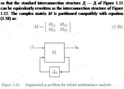
A structured model perturbation F 2 is introduced in the closed loop (see Figure 1.13). The transfer between w and z now corresponds to the LFT ЩМ, А2):

Fi(M, Д2) = Mu + МігДг(/ — M22A2)~l M21 (L43)

where M is partitioned as in equation (1.39).

Frequency и is fixed. Performance is guaranteed at this frequency despite the model uncertainty Д2 inside the unit ball BA2 if and only if:

(/) Robust stability of the closed loop is ensured:

/WM22 CM) < 1

(ii) The transfer between w and z remains lower than 1 despite the model uncertainty Д2:

max a(Fi(M{juj), Д2)) < 1 а2єв&2

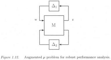
A fictitious full complex block Ді is added (see Figure 1.12). With reference to subsection 4.3, it can be remarked that:

a{Ft(M(juj),A2)) = (Fi(M(jw), Д2)) (1-46)

Let the augmented model perturbation Д of equation (1.38). Using the Main Loop Theorem, it can be claimed that the two above conditions are satisfied if and only if:

Мд(M(juj)) < 1 (1.47)

As a consequence, the robust performance problem reduces to an aug­mented robust stability problem, in which a fictitious performance block Дх is added (Doyle, 1985). Note that this block is possibly struc­tured: if signals w and z are decomposed as w = [uq,… ,wm]T and z = [zi,… ,zm]T, and if we are just interested in the transfer functions between scalar signals w% and z*, the performance block Дх will be chosen as a complex diagonal model perturbation.

Remark: equation (1.47) corresponds to a test ("Is robust performance guaranteed inside the unit ball ЯД2 ?"). As proved later, the compu­tation of the robustness margin (i. e. the maximal value of k, such that robust performance is guaranteed inside кВД2) is a skewed ц problem.

The Main Loop Theorem is introduced in the particular context of a robust performance problem. Note that this Theorem has been widely

used in many other contexts, and that it is the basis of many existing // results.

4.4.1

MAIN LOOP THEOREM

The standard interconnection structure M — A of Figure 1.11 is here again considered. The mixed model perturbation Д is split into two mixed model perturbations Д i and Д2:

(1.38)

Let Д і = 0 and Fi( M, Д2) the transfer between w and z on Figure 1.13. The following result is known as the Main Loop Theorem:

In the general case of a mixed model perturbation Д, no analytical expression of the s. s.v. /x(M) is available. Nevertheless, in the special

case of a single full complex block (resp. a single repeated real scalar), the s. s.v. fi{M) coincides with the maximal singular value a{M) (resp. the real spectral radius pr(M)).

When Д is a full complex block, p{M) = o(M). The small gain theorem provides indeed a necessary and sufficient condition of stability in the context of an unstructured model perturbation. In an alternative way, the following result can be used: if A is a complex matrix, the size of the smallest unstructured complex matrix Д, which renders the matrix A + Д singular, is a{A). In the context of the initial problem, matrix M is assumed to be invertible for the sake of simplicity. The singularity of I — MA is then equivalent to the singularity of M~l – Д. As a consequence, the size of the smallest unstructured complex matrix Д, which renders the matrix I — MA singular, is:

-(M ^ = W{M) = /ЁМ) (L34)

Consider now the case of a single real repeated scalar A = 6Ir. Then p(M) = pr(M), where the real spectral radius pr(M) is the magnitude of the largest real eigenvalue of M:

pR{M) = max{\i{M) / А,(М) € R)

PR(M) is zero if M has no real eigenvalue.

To prove that p{M) = pr{M), it suffices to note that the singularity of the matrix 1-М A implies the existence of a non zero vector x satisfying:

{I – 5M)x = 0 (1.36)

which can be rewritten as:

1/6 and x are thus an eigenvalue and eigenvector of M. 6 is moreover a real scalar, whose size is to be minimized, so that д ( A ( is the magnitude of the largest real eigenvalue of M.

Remark: in the same way, it can be proved that the s. s.v. /ід(М) coincides with the spectral radius p(M) (defined as the magnitude of the largest eigenvalue of M) when the model perturbation Д is a repeated complex scalar.

Д is now split as Д = diag(A,A2), where Ді and Д2 are two mixed structured perturbations. The skewed 1. 1.1. в( M) is defined as:

v{M) = 1 /тіп(к / ЗД = diag(Ax, к A2) with А j € BAj

and det(I — MA) = 0)

= 0 if no (k, Ді, Д2) exists (1-29)

When computing ц, the unit ball BA is expanded (or shrunk) by factor к until the matrix I – MA becomes singular for a structured perturbation inside кВА. When computing u, the unit ball BA2 (in the space of perturbations Д2) is expanded (or shrunk) by factor k, but the structured perturbation A remains now inside its unit ball ЯДі.

Proposition 4..1 illustrates that it is possible under mild conditions to

compute the exact value of v (resp. of /x) by computing recursively the exact value of д (resp. of д). When computing the exact value of u, it is moreover possible to use either a fixed point or a dichotomy search.

Proposition 4.. 1 Let mi the dimension of matrix Д*.

a/ if (Мп) < 1, then u(M) is the unique limit of the fixed point

iteration:

b/ if (Мц) < 1, then v(M) is the unique zero of the monotonous function:

c/ if Мд(М) > /хдх (Mu), then /хд(М) is the unique limit of the fixed point iteration:

Proof: see (Fan and Tits, 1992) for points a/ and c/ (with some technical arrangement because of the potential discontinuity of the mixed s. s.v.). Point b/ is deduced from point a/ using (a > 0):

/х(-Я) = -/x(tf) (1-33)

a a

Note however that u(aH) Ф av(H).

Remark: u(M) takes an infinite value if and only if /хд, (Мц) > 1 (Fan and Tits, 1992). It is indeed easily remarked that if /хд^Мп) > 1, then there exists a perturbation Д = diag(Ai,0) which renders the matrix 1-М A singular andsatisfies <т(Ді) < 1, so that v(M) = +oo. When ap­plying p, analysis to the standard interconnection structure M(s)-A(s), the nominal closed loop is assumed to be asymptotically stable, so that the s. s.v. vд(M(jut) ) can only take finite values. On the contrary, an infinite value can be obtained for the v measure.

The u> dependence is left out in the following: in the new interconnec­tion structure of Figure 1.11, the complex matrix M represents the value of the transfer matrix M(s) at s = ju>, while the model perturbation Д is an uncertain complex matrix, which also represents the value of the uncertain transfer matrix A(.s) at s = ju>. Remember especially that each block Az(s) of neglected dynamics becomes a full complex block Дг at s = ju).

A mixed structured perturbation Д is a free complex matrix with the following specific structure:

лС *C

, іЛ I, • • • , Д rri£

With classical notations (Fan et al., 1991), Д contains real scalars (which represent the parametric uncertainties), complex scalars Щ and full complex blocks ДJj7 Є Сктг+тс+‘>’ктг+гпс+ч (which represent the neg­lected dynamics). The integers mr, mc, me and kx define the structure of the perturbation. A real scalar (resp. a complex scalar 8flkmr+) is said to be repeated if the integer fc, (resp. kmr +l) is strictly greater than unity.

Д is said to be a complex model perturbation if it only contains com­plex scalars and full complex blocks. Conversely, Д is a real model per­turbation if it only contains real scalars. Д is finally a mixed model perturbation when it simultaneously contains real and complex uncer­tainties.

Remark: for the sake of completeness, the model perturbation Д above can also contain repeated complex scalars. Nevertheless, in many con­trol problems, Д only contains real (possibly repeated) scalars and full complex blocks. Specific problems however require the introduction of repeated complex scalars: see e. g. (Doyle and Packard, 1987) [5]. Note finally that a non repeated complex scalar can also be considered as a one dimensional full complex block.

The unit ball В Д is introduced in the space of the structured perturba­tion Д:

Note that the relation ег(Д) < 1 can be rewritten as and аД) В 1 . The s. s.v. is defined as:

liA(M) = l/min(k / ЗД Є кВА with det(I — MA) = 0) (1.28) = 0 if no (к, Д) exists

Remark: the notation дхд(М) emphasizes that this value simultan­eously depends on the complex matrix M and on the structure of the model perturbation Д. For the sake of simplicity, we will often drop out the Д dependence, i. e. simply note ц(М).

The notion of mixed structured model perturbation and the s. s.v. ц are formally introduced in the first subsection. The skewed s. s. s. s is defined

in the second one. The s. s.v. p, can be considered as an extension of classical algebraic notions, namely the spectral radius and the spectral norm (third subsection). The fourth subsection introduces the Main Loop Theorem in the specific context of robust performance problems. The notion of p sensitivity is defined in the fifth subsection. The last subsection presents in a qualitative way some difficulties arising when using the fj, framework.

Figure 1.10. Augmented и problem for robust performance analysis

In the spirit of #oo control, performance is achieved if a closed loop transfer matrix T(s) satisfies a frequency domain template а(ш) at all frequencies u>:

°{T{jш)) < a(u) (1.23)

Assume now the presence of uncertainties in the closed loop, so that T(s) is now an LFT Fi(M(s),A(s)) (i. e. the transfer between w and z in Figure 1.10). Д ( s) is most generally a mixed model perturbation, containing parametric uncertainties and neglected dynamics.

The nominal closed loop is assumed to satisfy the performance property at frequency a>, i. e. :

ff(Fi(W(j’w),0)) < а(ш) (1.24)

The robust performance problem consists in computing the maximal amount of uncertainties, for which closed loop performance is still achieved. The issue is thus to compute the maximal size of the mixed model per­turbation Д ( (s(. for which the following relation holds true:

<f(E,(M(jw), A(ju)) < a(u>) (1.25)

It will be seen in subsection 4.4 that this robust performance prob­lem can be equivalently transformed into an augmented robust stability problem, involving an additional fictitious full complex block (which is called a fictitious performance block). Chapter 7 will moreover illustrate that the robust performance problem is a skewed м problem rather than a classical ц problem.

Performance can be defined in two different ways. In the case of a real model perturbation, a first solution is to study the robustness of the location of the closed loop poles despite parametric uncertainties. In the general context of a mixed model perturbation, a second and more classical solution consists in checking whether a frequency domain template on a closed loop transfer matrix remains satisfied despite model uncertainties. In the first case, performance is rather defined in the time domain, whereas it is defined in the frequency domain in the second one.

2.3 n STABILITY

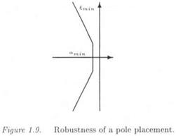
The special case of a real model perturbation Д is considered. As explained in section 2.1, the aim of /r analysis is to detect the crossing of one of the closed loop poles trough the imaginary axis. Assuming that the nominal closed loop poles lie inside the left half plane, the idea is to compute the s. s.v. fi(M(s)) on the border of this left half plane (namely the imaginary axis), and to compute the robustness margin kmax with equation (1.22).

More generally, the singularity of the matrix I — AM(sq) is equival­ent to the presence of a closed loop pole at the point so of the complex plane. As a consequence, robust stability inside generic regions ft of the complex plane can be studied: assuming that the nominal closed loop poles belong to ft, it suffices to compute the s. s.v. along the border of ft to find the minimal size real model perturbation, which shifts one closed loop pole on this border.

ft may be the unit disc in the case of discrete time systems, or a trun­cated sector in the continuous-time one (see Figure 1.9). Performance is indeed defined in this context by minimal values £TOjn and amm for the damping ratio £ and the degree of stability a [4]. To some extent, these specifications correspond to requirements on the rise time and overshoot of the closed loop step response, or on the time needed to reject an unmeasured disturbance or a non zero initial condition.

An important practical issue is the choice of weights on model un­certainties. It was seen in subsection 1.2 that a template is to be de­termined for each block of neglected dynamics. Consider now the case of parametric_uncertainties 6{. Each is assumed to belong to an in­terval [—ві, ві]. The normalized parametric uncertainties 8{ are then introduced as

Let kmax the robustness margin: the parametrically uncertain closed loop remains asymptotically stable for each 8{ Є [—kmax, kmax], or equi­valently for_each ві Є [—kmax ві, kmax ві]. The choice of the initial intervals [—ві, ві] is critical, as illustrated by the example of Figure 1.8, with only two parametric uncertainties ві and в2. The zero point cor­responds to the nominal values of the uncertain parameters: remember that the nominal closed loop system is asymptotically stable. The space of parametric uncertainties ві and 62 can then be split into two subdo­mains. In the first one, which contains the zero point, the parametrically
uncertain closed loop remains asymptotically stable. In the second one, this closed loop is unstable. At the limit between the two subdomains, the closed loop is marginally stable.

Generally speaking, the ц approach provides the largest hypercube in the space of the normalized parametric uncertainties Si, inside which the closed loop stability is guaranteed. This hypercube becomes a box in the space of the initial parametric uncertainties 0*. What illustrates Figure 1.8 is that various stability boxes are obtained depending on the choice of the initial intervals [—&i, 0i.

Obviously, the above discussion can be extended to the general case of a structured model perturbation containing parametric uncertainties and neglected dynamics: various stability domains are obtained depending on the choice of the weights on the parametric uncertainties and neglected dynamics. We will come back to the study of this important issue in the following.