Category A PRACTICAL. APPROACH TO. ROBUSTNESS. ANALYSIS

In the general case of mixed uncertainties, (Fan et al., 1991) first formulate the problem of computing the exact value of //as a smooth constrained optimization problem. The result is then used to derive a computable p upper bound, in which a maximal generalized eigenvalue is to be minimized with respect to the sets V and Q of scaling matrices (see the previous subsection).

An other approach for computing a /t upper bound is proposed by (Safonov and Lee, 1993). This method basically uses the positivity the­orem: the interconnection structure M — A is first transformed, so that the new feedback uncertainty block becomes positive (using a bilinear transformation). The conservatism of the positivity theorem is then minimized with multipliers. The optimal value of these multipliers is here again obtained as the solution of an LMI problem.

Both methods in (Fan et al., 1991; Safonov and Lee, 1993) solve in a more efficient way the problem of (Doyle, 1985), in which a p up­per bound was proposed for the case of non repeated real scalars. As noted in (Safonov and Lee, 1993), the two upper bounds in (Fan et al., 1991; Safonov and Lee, 1993) are equivalent for this case. The equival­ence can be further characterized using a result in (Haddad et al., 1992) (Corollary 2, p. 2819).

The j upper bound above does not account for the real nature of the parametric uncertainties, so that this upper bound is called "a complex /л upper bound": real and complex scalars are indeed treated in the same way in the structure of the scaling matrix D. An additional scaling

matrix G can take into account the specificity of scalars <S[. G must belong to:

G — {G — diag(GGmr, 0^m 0^

with Gi = G* Є Cki’ki} (5.14)

The complex p upper bound of the previous subsection is recovered with G = 0 (see equations (5.12) and (5.13)). On the other hand, the new quasi convex and non differentiable optimization problem can be solved,

either using a general LMI solver (the issue is to minimize a maximal generalized eigenvalue), or using the specific structure of the optimiza­tion problem.

Indeed, an alternative formulation of the above mixed p upper bound was proposed in (Young et al., 1995). The following sets of scaling matrices are associated to Д (IV = 5Y=ri &i):

^ — diag(D 1,…, Dmr+mc j d Jfemr+mc+i > •

with det(Di) фО, Dte CkiM, dj ф 0 and dj Є C} g = {G = diag(gi,…,gN, Okmr+I,…,Okmt,+mc+mc) with gj Є R} (5.16)

D Є V is consequently a positive definite matrix, unlike D Є V. G Є G is an hermitian block diagonal matrix unlike G Є Q, which is a real diagonal matrix. The following Lemma is extracted from (Young et al., 1995).

1 — jG)F~^4) < 1

then p(M) < /3.

Remark: roughly speaking, the /.t upper bound proposed in the above Lemma involves the minimization of a maximal singular value, whereas the p upper bound of (Fan et al., 1991) involves the minimization of a maximal generalized eigenvalue. These bounds are nevertheless identical (Young et al., 1995): see Lemma 2..1 of chapter 10.

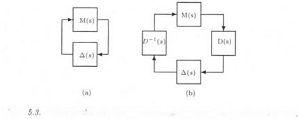
Introduction of D scales in the standard interconnection structure

The standard interconnection structure M(s) — A(s) of Figure 5.3.a is considered. A p upper bound at frequency u> is directly provided by the small gain theorem (M = M(juj)):

p(M) < o(M) (5.8)

This theorem does not account for the structure of the model perturba­tion A(s). To this aim, a scaling transfer matrix l)(s) is used to decrease

the conservatism of the /л upper bound (5.8) (Safonov, 1982). D(s) must commute with A(s), i. e.:

D~1{s)A{s)D{s) = A{s) (5.9)

D(s) can thus be introduced into the interconnection structure without modifying the stability properties of the closed loop (see Figure 5.3.b).

Frequency и is fixed: let then D = D(ju) and M = M(jiv). Re­member that the structure of the model perturbation A is (see equation (1.26)):

where J[ and Jj are real and complex scalars, while Д^ Є Ckrnr+mc+4,kmr+m<:+’> is a full complex block. Because of equation (5.9), the scaling matrix D must belong to:

, Dmr+mc i + i ) ■ * • > dmc ^mr-fmc+mc )

with Di = D* >0,Die Cki’ki and dj > 0} (5.11)

The new fj. upper bound is:

ц(М) < mf^a(DMD~l)

The issue is thus to minimize the conservatism of this upper bound by finding the optimal value of D, which minimizes a{DMD~l). This con­vex and non differentiable optimization problem can be solved in numer­ous ways: see (Doyle, 1982; Safonov, 1982; Packard and Doyle, 1993) and included references.

Remark: this jr upper bound can be rewritten as1:

This is an LMI problem involving the minimization of a maximal gener­alized eigenvalue.

1.2 INTRODUCTION TO LMIs

A Linear Matrix Inequality (LMI) is an inequality constraint A(x) < 0, where A(x) is an hermitian square matrix (A(x) = A*(x)) depending linearly on the vector x of parameters:

N

A(x) = A0 + ^2 АіХі

i=i

Matrices Ao and A are fixed. Various techniques and softwares (Boyd et al., 1994; Gahinet et al., 1995) are available for solving the feasibility problem: does there exist a value of vector x for which the relation A(x) <

0 holds true ?

_ Let two hermitian matrices A and B, with В > 0. the quantities (A, B) andry(i4, B) are defined as:

A(A, В) = sup(7 Є R : det(A — 7B) = 0)

p(A, B) = sup(j Є R : (A — jB) > 0) (5-7)

where A(M) denotes the maximal eigenvalue of a matrix M. r](A, B) is almost always equal to the maximal generalized eigenvalue A(A, B), except possibly when r](A, B) = 00 (see Proposition 5.1.c of (Fan and Tits, 1992)).

Let A(x) and B(x) matrices which linearly depend on vector x. The minimization of A(A(x),B(x)) is a quasi-convex optimization problem, which can be recast as the minimization of scalar 7 under the LMI constraint A(x) — yB(x) < 0. A first simple solution is a dichotomy

search over 7: for a given value of 7, the feasibility problem "does

there exist a value of vector x satisfying A ( x ) — jB ( x ( < 0 ?’ 1 is to be solved. More sophisticated solutions, involving the direct minimization of A ( A(—) , A(—(), are also available (Gahinet et al., 1995).

This method, which provides a real ц upper bound, is based on linear algebraic manipulations and on the properties of the determinant (Jones, 1987). An upper bound of ц{М) is obtained as:

. DMD-l<t> + (DMD~4)

mm max A(———————– 1——————- )

D Ф v 2

where A* denotes the complex conjugate transpose of A, A (A) is the largest eigenvalue of A, D is a real diagonal scaling matrix and Ф is a permutation matrix, defined as Ф = diag(± 1,±1,…). Since there are 2n matrices Ф to be considered in the case of an и dimensional vector S of parametric uncertainties, the method is here again exponential time.

This upper bound is proved in all cases to be less conservative than the upper bound of the complex s. s.v. of subsection 2.2. Note that the per­mutation matrix Ф may indicate a direction in the space of uncertainties which leads to instability.

This method, which provides a real p lower bound, is based on a conjecture about the structure of the minimum norm parameter per­turbation (Dailey, 1990). Assume that all but two components Si and Sj of the minimum norm parameter perturbation achieve the maximal magnitude k:

6[ = ±k VI ф і and VI ф j (5.3)

Rather than solving the general equation with respect to the vector of parametric uncertainties:

det(I — diag(S)M) = 0 (5.4)

it suffices now to solve it with respect to the two free components Si and Sj, and this reduces to finding the real roots of a set of two quadratic
equations in Si and Sj: remember indeed that Mis complex, so that the above equation has generally a single solution in Si and Sj. If the abso­lute values of the obtained Si and Sj are less or equal to k, a destabilizing parameter perturbation 5 with norm к has been obtained.

Relation (5.3) defines a two dimensional face of the hypercube kD, so that the above operation has to be done on each such face of the hypercube. The method, which is thus exponential time because of the exponential growth of the number of two dimensional faces as a function of the number of parametric uncertainties, is nevertheless easy to imple­ment. The technique provides a lower bound of real /і, since the counter­examples in (Holohan and Safonov, 1993; Ackermann, 1992) prove that it can not be assumed in the general case that more than one component Si of the minimum norm parameter perturbation achieves the maximal magnitude.

Methods are described in this chapter for computing bounds of the real, complex or mixed s. s.v. /хд(М). Remember that M denotes in the following a complex matrix, which may correspond to the value of the transfer matrix M(s) at s = juj.

1. COMPUTATION OF THE REAL S. S.V.

The specific case of a model perturbation Д = diag(S), which only contains real non repeated scalars Si, is considered in this section.

1.1 A SOLUTION BASED ON THE MAPPING THEOREM

The definition of the unit hypercube D is first recalled:

D = {<5 = [Si… Jn] I Si Є R and |^| < 1} (5.1)

The s. s.v. g,, or its inverse the multiloop stability margin (m. s.m.) km, is defined as:

km — — = min(k I Є D s. t. det(I — kdiag(S)M) = 0) (5.2)

M

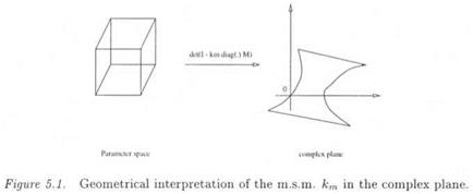
The m. s.m. km can thus be interpreted as the lowest value of k, such that the image of the unit hypercube D by the operator det(I – kdiag(S)M) contains the origin of the complex plane (see Figure 5.1 – this image is called a value set).

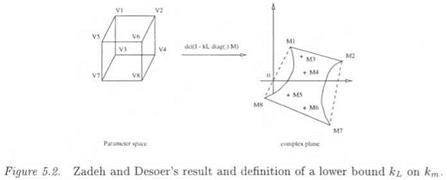
However, building this image is generally a computationally infeasible task. Nevertheless, in the special case of a model perturbation Д contain­ing only non repeated real scalars Si, the operator dei(I – kdiag{S)M) is a complex multilinear function of vector S. It is thus possible to use a result in chapter 9 of (Zadeh and Desoer, 1963), which claims that the image of the unit hypercube D by the operator det(I – kdiag(S)M) is contained in the convex hull of the images Mi of the vertices Vi of D (Mapping Theorem). A lower bound ki of the m. s.m. km can thus be obtained as the smallest value of k, for which the convex hull contains the origin (see Figure 5.2).

Remarks:

(/’) The approach is exponential time, since an hypercube has 2” vertices when n parametric uncertainties Si are considered.

(ii) Like Zadeh and Desoer’s result, Kharitonov’s and edge theorems (Barmish and Kang, 1993; Bartlett et al., 1988) can also be interpreted in a frequency domain approach as Zero Exclusion Tests (Barmish and Kang, 1993). The difference between these three theorems is the way the uncertain parameters enter the plant model.

(iii) In the special case of a real matrix M (this especially occurs at the zero frequency, i. e. when M is the DC gain of the transfer matrix M(s)), the result by Zadeh and Desoer provides the exact value of the m. s.m. km. The convex hull coincides indeed with the image of the unit hypercube D by the operator det(I – km diag(S)M), since both sets he in the real axis.

The result by Zadeh and Desoer was used in (DeGaston and Safonov, 1988) as the basis of a computational algorithm, which provides the exact value of real ц using a branch and bound scheme. The idea is to partition the unit hypercube into a set of smaller hyperrectangles, and to apply Zadeh and Desoer’s result on each of these hyperrectangles, in order to decrease the conservatism of the lower bound кь of km. An upper bound of km (i. e. a p lower bound) is also computed to stop the partitioning process, when the gap between the bounds is sufficiently small: see (De – Gaston and Safonov, 1988; Ferreres et al., 1996a) for further details.

Remark: the algorithm in (DeGaston and Safonov, 1988) can be sum­marized in 3 operations, computing the lower bound, computing the upper bound and partitioning. Other algorithms with the same branch and bound structure were developed in (Chang et al., 1991; Balakrishnan et al., 1991; Newlin and Young, 1992). However, the aim of the algorithm in (Newlin and Young, 1992) is not to compute the exact value of mixed p, but rather to reduce the gap between the bounds to an acceptable value (typically 20 %), thus limiting as much as possible the exponential growth of computation with the number of uncertainty blocks (remember the problem of computing the exact value of p is NP hard).

Uncertainties are introduced in the natural frequencies of the 6 flexible modes. A real modal state-space representation of the flexible model is used. If the method of chapter 3 (section 4.) is applied, the flexible LFT model contains 6 twice repeated real scalars. Otherwise, if the method of subsection 2.2 is used, the LFT contains 6 non repeated real scalars.

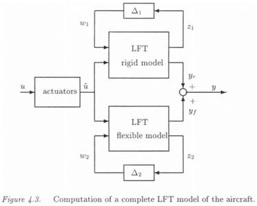
The complete LFT model у = Fi(H(s),A)u is simply computed by adding at the physical outputs yr and уf the rigid and flexible LFT mod­els (see Figure 4.3): remember indeed that the interconnection of LFTs is an LFT. Д = diag(/S. i, Д2), where Д; is a real model perturbation con­taining 14 real non repeated scalars (corresponding to uncertainties in the 14 stability derivatives). Д2 is a real model perturbation containing, either 6 real twice repeated scalars, or 6 real non repeated scalars (cor­responding to uncertainties in the frequencies of the 6 bending modes).

An alternative method to the approach of chapter 3 (section 4.) is presented for introducing uncertainties in the frequency of the bending modes. Let ші and & the natural frequency and damping ratio of the ith flexible mode. When reducing the real modal state-space representation to this single mode, one obtains :

An uncertainty in the natural frequency ші is introduced as:

— (1 + Si)u>oi (4-12)

where u>oi denotes the nominal value and Si the associated relative vari­ation. Assuming that the damping ratio and frequency variation are

small (i. e. £; <£. 1 and |<5*| 1), the dynamic matrix can then be ap­

proximated as follows:

—2£ja>oi — (1 + 2<5;)a>o;2
1 0

ДА; is a rank one matrix, which is factorized under the form ДА; = —MiSiNi. The uncertainty can hence be expressed as a feedback of gain Si between the scalar fictitious input e/ and output z/ :

A possible choice for M; and iV; is :

1.2 THE RIGID LFT MODEL

We come back to the problem of chapter 2 (subsection 1.1), and note first that the 14 stability derivatives enter in an affine way the state-space equations (2.1), (2.2) and (2.3) of the aerodynamic aircraft model. The LFT model can thus be computed with Morton’s method.

Note that the parametric uncertainties in the stability derivatives could be directly introduced in the physical model, as in the missile case. Nevertheless, it is simpler here to apply Morton’s method, because of the complexity of the aerodynamic equations (2.1), (2.2) and (2.3).

It is moreover interesting to emphasize that the 14 stability derivat­ives enter as rank-one model perturbations the state-space aerodynamic model, even when these coefficients simultaneously enter the state matrix A and output matrix C (this is e. g. the case of Yp). When considering the jth uncertain parameter, this means that the corresponding matrix Pj in equation (3.5) is a rank one matrix, so that the associated real scalar Sj is non repeated.

As a consequence, the LFT model of the rigid transport aircraft con­tains 16 inputs (2 physical inputs and 14 fictitious inputs) and 18 outputs (4 physical outputs and 14 fictitious outputs). The associated model perturbation contains 14 non repeated real scalars. This LFT model is minimal.