Category AIRFOILS AT LOW SPEEDS

Comments on Airfoils

In this section the performance of each airfoil is discussed in detail. Emphasis is placed on highlighting the important characteristics with respect to the other airfoils. Following these comments, smaller sections discuss:

(1) stall behavior

(2) trips and surface roughness

(3) trailing edge thickness

(4) surface waviness and contour accuracy.

In some of the airfoil discussions we give examples of sailplane performance in order to compare one airfoil with another. It should be noted in these examples that while one airfoil may be good for a particular configuration, it does not necessarily follow that it is good for all configurations. This is one of the reasons why there are so many “favorite” airfoils. In light of this, the reader is left to make the final decision as to which airfoil is best suited for a particular sailplane. To this end, a computer and an accurate performance prediction program are invaluable aids in the airfoil/aircraft integration process.

Even though most of the discussions are related to the RC sailplane, the airfoils are by no means restricted to this use. Furthermore, the aerodynamic phenomena described are common to all airfoils operating at low Reynolds num­bers.

Many of the airfoils tested were jiot originally intended for use on RC sail­planes, but have come to be used for this application by trial and error. On the other hand, the new SD-airfoils (as well as the DF-series) were designed for the RC sailplane. Rather than tailor a design to one, particular aircraft, the SD-series airfoils were designed for different, general classes of flying; for example, thermal-duration, F3B, multi-task, etc. Additional improvements in performance can probably be made by properly integrating the initial airfoil design process into the overall aircraft design24.

Some miscellaneous notes follow:

(1) For several of the airfoils camber-changing flaps are recommended for best per­formance. In these cases, “flaps” and “full-span flaps” and “camber-changing flaps” are used interchangeably.

(2) At the end of each airfoil discussion is a list of related airfoils given in order of decreasing similarity to aid the reader in the selection process.

(3) As previously mentioned in Section 2.2.3, the designation “-PT” (for Prince­ton Tests) is used after the names of the actual airfoils tested to distinguish them from the nominal or ideal airfoils. Depending on the accuracy of the wind tunnel model, one may chose to build using the actual coordinates (with the PT-designation) listed in Chapter 7 for this purpose. Also, the actual co­ordinates should be used for any theoretical computations, since in some cases the deviation from the nominal is large.

(4) The nominal Reynolds number is used in the labels of the airfoil polar plots while the actual Reynolds number is listed with the tabulated data.

(5) The airfoil maximum thickness and camber is listed at the end of each airfoil discussion for quick reference; they are also listed in tabular form in Chapter 9.

(6) If two or more models of the same airfoil were built, the designation А, В, C, etc. is used to indicate the different models. In some cases the versions may differ by the type of surface finish, the addition of a flap, or some other major modification.

(7) In addition to testing the plain airfoils, the effects of a number of different boundary layer trips were examined in a search for improved performance. Figure 13.7 shows the geometry of the plain, zig-zag, bump, and blowing trips. Note that the trip “type” designations А, В, C, etc. should not be confused with the model “version” designations А, В, C, etc.

(8) Airfoil moment data were not taken. For an estimate of the moment about the quarter-chord point, Chapter 8 lists the average moment coefficients over the range 0.2 < Ci < 0.8 for Rn of 200k for some of the airfoils, as predicted by the Drela and Giles ISES code.

(9) Airfoil polars and lift plots are given separately in Chapter 12.

(10) An abbreviated description of the trips is found in the figure titles. These abbreviations have the following meanings:

u. s. upper surface

u. s.t. upper surface trip

l. s. lower surface

l. s.t. lower surface trip

z/c normalized trip position measured from the model leading edge to the trip leading edge h/c normalized trip height

w/c normalized trip width.

When the trip type is not explicitly stated, the trip is the simple two-dimen­sional trip strip. For example see Fig. 12.22.

(11) Although some of the discussions of the airfoils deal with the effects of bubble ramps, these are not important with regards to building and actually using the airfoils. Therefore, no specific details of the ramps are provided and airfoil velocity distributions are not given.

(12) There are plots comparing the nominal and actual airfoils (termed here “digi­tizer plots”) in Chapter 10, and plots comparing different nominal and actual airfoils in Chapter 11.

(13) The data used in generating the polar plots is tabulated in Chapter 13 and is keyed according to the airfoil name and figure number. The data is ordered as it appears in the figure title.

(14) The aircraft polars in this chapter were made with SAILPLANE DESIGN, a computer program (available from Fraser) for evaluating and comparing sailplane performance. Although SAILPLANE DESIGN allows the user to vary any parameter, the polars presented here compare aircraft that are iden­tical except for the airfoil and weight. The configuration is shown on the graph. The profile drag of the wing is taken from the tunnel data and the induced drag is calculated using lifting line theory15 for both the wing and horizontal stabilizer. The fuselage and empennage profile drags are calculated using equation 5.18 of Reference 15. No allowances are made for parasitic drags nor is any correction applied for a non-elliptical lift distribution. (The former are impossible to accurately quantify and the latter would be very small in any case.) Neither is significant when comparing similar aircraft. The three sloping lines are lines of constant sink speed: 1.0, 1.25, and 1.5 ft/s. All units are feet, pounds, seconds.

Project Design Methods and Goals

Three main tools were used to design new airfoils: the Eppler and Somers design code20, the ISES code written by Drela and Giles21’22, and the wind tunnel described previously. The Eppler and Somers code formulates the design problem in a way that allows quick and easy manipulation of the airfoil shape. With a minimum number of parameters, almost any desired velocity distribution can be obtained. However, because this code does not accurately predict the performance of airfoils in the Reynolds number range considered here, it was used mainly to obtain the inviscid velocity distributions and to give an estimate of the transition point behavior.

The ISES code solves the two-dimensional Euler equations coupled with a momentum integral boundary layer formulation using a global Newton method. Over the Reynolds number range considered in this investigation, it predicts airfoil performance more accurately than the current version of the Eppler and Somers code. In particular, the agreement with the experiment at Reynolds numbers of 200k and greater is very good. However, the agreement depends on the choice of the n value used in the en transition criterion. While the ISES code provided a relatively good estimate of the performance, wind tunnel results were the ultimate test of an airfoil.

The design approach was to generate an airfoil with the desired inviscid ve­locity distribution using the Eppler. and Somers code, and then predict the per­formance at a Reynolds number of 200k using the ISES code. If the performance was poor, the new airfoil was redesigned and the process repeated. Upon reach­ing a suitable design through this iteration process, a wind tunnel model was built and tested. Based upon the wind tunnel results, the new airfoils were further refined and the process repeated.

Before discussing airfoil design, it should be pointed out that for any aircraft in straight and level flight the relation between C and chord Reynolds number is given by:

Rn <x

This relation emphasizes the fact that the Сд should be minimized for a value of Ci and the corresponding Rn. Thus, the optimum airfoil design is clearly dependent upon the configuration and desired tasks of the aircraft for which it is designed. The designs discussed below are based upon RC sailplane
configurations; however, the general principles apply to any type of low-Reynolds number aircraft.

A popular RC soaring, cross-country airfoil is the E374. It is commonly used on aircraft intended for high speeds, with relatively little importance placed on the performance at low speeds. The experimentally determined drag polars for this airfoil are shown in Figs. 12.24-12.29. This airfoil works well at high speeds because of the small values of the drag coefficient at the higher Reynolds numbers throughout a range of low C values. At lower Reynolds numbers, the drag increases dramatically as C moves from 0.0 to 0.5, and then decreases from 0.5 to 0.8. This behavior indicates the formation of a large laminar separation bubble on the upper surface.

The inviscid velocity distribution about the E374 for a Ci of 0.55 is shown in Fig. 4.1. A “kink” in the upper-surface velocity distribution beginning at 40% separates it into two distinct regions. Over the forward 40%, the velocity changes little, and the majority of recovery takes place over the aft 50% with a relatively strong adverse pressure gradient. At low Reynolds numbers, this pressure gradient results in a large laminar separation bubble. To reduce the drag, the pressure gradient should be reduced. However, if the same pressure differential is to be recovered, then the recovery region must start farther up­stream, as shown by the dashed line in Fig. 4.1. This longer region of smaller adverse pressure gradient is termed a bubble ramp. Before this point is discussed further, it is important to observe the behavior of the transition point on the upper surface with increasing Ci.

As a result of the kink in the velocity distribution at 40% chord, the transition point moves rapidly forward with C as shown in Fig. 4.2. (Of course, transition does not occur at a point but rather over some finite distance.) In this case the point refers to the location at which transition was predicted to occur by the Eppler and Somers code using a method based on the boundary layer shape factor for Rn of 200,000. Knowledge of the shape of the transition-point curve is helpful when designing with the Eppler and Somers code because it is similar to the distribution of design parameters which specify the airfoil (a* with i/)20. In the “redesign” of the E374, the kink in the velocity distribution was removed to define a new airfoil—the SD6060. The resulting transition point behavior and velocity distribution are shown by the dashed lines in Figs. 4.1 and 4.2, respectively. Removing the kink shifted the transition point farther forward for Ci greater than 0.5. In this case, separation will occur earlier because of the steeper initial gradient, but with the transition point farther forward, the separation bubble will be shorter and the drag will be lower.

A comparison between the experimentally determined drag polars for the E374 and SD6060 is shown in Fig. 4.3. There has been a reduction in drag throughout the central portion of the polars for all Reynolds numbers because the bubble ramp has reduced the length of the separation bubble. (Some of this

reduction in drag is due to a thinning of the airfoil; the E374 is 10.9% thick and the SD6060 is 10.4% thick.) In addition to the decrease in drag in the central region, the increase in drag as Ci approaches 1.0 is more gradual in the case of the SD6060, which is consistent with the smoother forward movement of the transition point.

A further example illustrating the effectiveness of a bubble ramp in the upper – surface velocity distribution can be seen by comparing the E205 and the S302123. The E205 is usually used as a “multi-task” airfoil because of its relatively good performance at both high and low lift. This airfoil has an upper-surface velocity distribution which is similar to the E374 in that it also contains a kink. The velocity distribution of the S3021 is essentially the same as that of the E205 except the kink has been replaced with a bubble ramp as in the SD6060. Figure

4.4 shows a comparison between the drag polars of the E205 and S3021 at several Reynolds numbers. The differences are similar to those noted between the E374 and SD6060, that is, at all Reynolds numbers the drag of the S3G21 is lower than that of the E205 in the central region of the polars. However, at the highest Reynolds number (300k) the E205 has lower drag than the S3021 for Ci = 0.9. As discussed earlier, as the speed increases, the lift coefficient decreases so that for typical low Reynolds number configurations, at 300k the lift coefficient would be considerably less than 0.9. Thus, for low Reynolds number aircraft, the S3021 will perform better than the E205.

These examples illustrate that significant improvements can be made over existing designs by relatively minor changes in the velocity distributions (which, of course, directly alter the airfoil shape). Other airfoils, such as the SD70Q3, demonstrate that if sufficient attention is paid to the control of the bubble, it is possible to design entirely new, low Reynolds number airfoils that show little or no evidence of increased drag due to the bubble, even at 60k. What is not known at this "point is how far this design philosophy can be “pushed”. Even though improvements have already been demonstrated, the optimum shape and location of the ramp remain to be determined. Employing airfoils with bubble ramps on model aircraft will provide further insight into the benefits of this type of design and will help guide further study.

E205B-PT and S3021A-PT

и Rn = 100,000 – E205B-PT v Rn = 300,000 ^ Rn = 100,000 – S3021A-PT д Rn = 300,000

Airfoil Hysteresis

The term hysteresis, as applied to airfoil aerodynamics, means the difference in C;, Cdy or Cmc/i at a given angle of attack when this angle of attack is approached from a higher and then a lower value. This behavior may be seen in the in the Ci vs a plot. See for example Fig. 12.2. In cases with hysteresis, as the angle of attack is increased from zero to stall, the Cj will usually reach a maximum value and then drop off at some particular a. However, when a is decreased, the C will not retrace its original curve; rather it will stay at the “stall” Ci until a is somewhat below the previous stall value, and then suddenly jump up to rejoin the original Ci vs a curve. Hysteresis in the aerodynamic coefficients with both Reynolds number and angle of attack is common to many of the airfoils tested.

Invariably, hysteresis is a sign of a large, laminar separation which in turn yields high bubble drag. Since this effort concentrated on those airfoils with low bubble drag, the detailed effects of hysteresis were not closely examined. In general, airfoils with hysteresis in the middle of the I2n-envelope of the aircraft should be avoided.

44 Airfoils at Low Speeds


Trips and Bubble Ramps

Several means can be used to destabilize the laminar boundary layer and promote an early transition. The most direct means of doing this is through the airfoil shape. At higher Rni than those found on model aircraft, a short, gradual pressure recovery, called a transition or instability ramp, is sometimes used before the steeper main recovery. The purpose of the ramp in this case is to ensure that the boundary layer is fully turbulent and energetic before reach­ing the main pressure recovery. At low Rn, the transition ramp is still useful, although it needs to be longer, and may be more appropriately called a “bub­ble” ramp. The gradual pressure recovery of the ramp in this case shortens the length of the bubble by shortening the distance required for reattachment. As the Rn decreases, more and more of the airfoil surface is required for the bubble ramp18’19. In fact, for a Rn near 60k and at moderate lift coefficients, almost the entire upper surface of the airfoil is needed to ensure transition and subsequent reattachment.

Another method of inducing transition is through the use of a turbulator or trip. Typically, these are external ridges or bumps applied to the surface of the airfoil in a direction parallel to the span. They protrude into the boundary layer in such a way as to energize it sufficiently to promote transition. Many free-flight model aircraft employ turbulators to improve performance. Several detailed experiments, as summarized by Mueller4, have amply demonstrated that if an airfoil has high drag and hysteresis owing to a laminar separation bubble, a turbulator often alleviates these adverse effects by shortening the length of the bubble.

Currently at issue in the design of low Reynolds number airfoils are the fac­tors governing the use of bubble ramps and turbulators. At very low Reynolds numbers, turbulators may be better them bubble ramps, but as the Rn increases, the bubble shortens naturally. Thus, the turbulator becomes unnecessary and handicaps the performance by making transition happen too early. In this case the ramp would probably be better. In the middle of the low-iEn range, the ques­tion remains unclear. Is it better to use only a bubble ramp or only a turbulator or a combination of both? Usually airfoil turbulators are simple two-dimensional strips, but some three-dimensional trips (such as zig-zag tape and bump tape) have proved highly successful in application to modern, full-size sailplane airfoils. In our research, trips and ramps were used to begin to explore their respective benefits and operating regimes.

Low Reynolds Number Terminology

The concepts of modern airfoil design and the attendant jargon are famil­iar mostly to specialists. In addition, some of the terms commonly used even by aerodynamicists have modified or expanded meanings when applied to low Reynolds number airfoils. For example, the concept of a bubble ramp is derived from a transition ramp, but they are not synonymous. To assist the general reader and to avoid confusion we here define those terms that are specific to low Reynolds number aerodynamics in order to supplement what can be found in textbooks15’16. We also have gone into greater detail in the earlier airfoil discus­sions in Section 5.1 so that the concepts will be familiar when they are referred to more briefly In the later ones.

3.1 Laminar Separation Bubbles

As described in Chapter 1, laminar separation takes place at low Rn due to the reluctance of the boundary layer to make a natural transition from laminar to turbulent flow on the airfoil surface. This type of separation and the subse­quent formation of a laminar separation bubble are the principal reasons for the degradation in airfoil performance with decreasing Rn.

At high Rn (greater than 1 million) a graph of С/ vs Cd for most airfoils shows a rounded appearance with the convex side towards the C axis. See References 15 and 17 for examples of polars at higher Rn’s. At low Rn the situation is often markedly different. Here, separation is a major factor and can contribute a large increment of drag not normally found at higher Rn’s. The effect on the shape of the polar is to produce a bulge in the mid-Cf range that is concave towards the C axis (see Fig. 12.13). Interestingly, with increasing Ci the drag decreases again just before stall.

Because of these effects, the shape of the polar clearly reveals the severity of the laminar separation bubble. For example, the E214 has a major problem with this at Rn’s of 60k and 100k. (This will be discussed in Section 5.1.) If one compares the tripped and untripped cases (Figs. 12.19 and 12.22) the difference in shape illustrates the difference in the separation—the polar changes from concave for the untripped (separated) case, to a more favorable convex shape for the tripped case.

Separation can, however, be minimized by proper design. For such airfoils, e. g. the SD7003, the graphs, even without trips, are more typical of those for higher Rn’s.

Comparison with Other Facilities

Measurements in other facilities can provide a basis of comparison for the lift and drag obtained in this project. Unfortunately, it is difficult to make a broad range of’systematic comparisons because relatively few of the airfoils tested in this project have been tested in other facilities at the same Reynolds numbers. Until recently the primary application for airfoils operating at Reynolds numbers considered here was for model aircraft. Consequently, little effort was directed at designing and testing airfoils in the Reynolds number range 60к < Rn < 300&. The majority of available data with which to compare the Princeton data is from the Model Wind Tunnel at Stuttgart7,3’10; however, comparisons were also made to data obtained from NASA Langley11, Delft8’12, and Notre Dame13’14.

Comparisons of the available drag polars are shown in Figs. 2.9 through 2.20, and comments are provided in several cases. A listing is given at the end of the discussion.

Fig. 2.10 compare drag polars obtained in the Princeton tunnel (using the E205B-PT model) with those in the Delft tunnel8 and in the Model Wind Tunnel at Stuttgart7 for the E205 at Reynolds numbers of 60k, 100k, and 200k. At 200k all three facilities agree to within 10% over the central region of the lift range. The agreement between Delft and Princeton data at 100k is also quite good. However, at 60k the agreement is worse.

Stuttgart tests of the S3021 in 1986 are compared to the Princeton data in Fig. 2.20 for Reynolds numbers of 100k and 200k. Overall agreement is rea­sonable; however, the Princeton drag values are generally lower. A comparison with Stuttgart data from 1980 on the NACA 0009 is shown in Fig. 2.18. In this case, the Stuttgart data indicates lower drag throughout much of the lift range. Results of the S2091 are compared with Stuttgart (1986) in Fig. 2.19.

At Reynolds numbers of 100k and below, the agreement is poor, with Stuttgart generally finding higher drag. By 200k, the agreement is quite good.

Comparisons were also made with data from Notre Dame as shown in Figs. 2.16 and 2.17. In the case of the FX63-137, the Notre Dame data indicates a significantly higher drag than either the Stuttgart or Princeton values.

Fig. 2.13 shows a comparison of the E387 data from the present work to that from the NASA Langley11, Delft12, and Stuttgart9. Note that the E387 model used in the Princeton test (E387A-PT) is decambefed (see Fig. 10.13) which is reflected by a shift in the polar to lower lift values. The camber error is approximately 0.4%. Nevertheless, the general agreement between the data from the NASA Langley, Delft, and Princeton is good.

The discrepancies found in these comparisons are primarily due to differences in (1) flow quality, (2) accuracy of measurements, (3) methods of measurement, and (4) model accuracy. At this time it is difficult to determine how much of the disagreement is due to each of these areas, but we have documented those of the present project to allow for future comparisons.

Fig. 2.9 CLARK-Y-PT vs CLARK-Y (Althaus, 1980)9

Fig. 2.10 E2Q5B-PT vs E205 comparisons 7,8

Fig. 2.11 E214B-PT vs E214 (Althaus, 1986)7

Fig. 2.12 E374B-PT vs E374 (Althaus, 1985)10

Fig. 2.13 E387A-PT vs E387 comparisons s>11>12

Fig. 2.14 FX60-100-PT vs FX60-100 (Althaus, 1980)9

Fig. 2.15 FX63-137B-PT vs FX63-137 (Althaus, 1980)9

Fig. 2.16 FX63-137B-PT vs FX63-137 (Bastedo and Mueller, 1985)14

Fig. 2.17 M06-13-128-PT vs M06-13-128 (Pohlen and Mueller, 1983)13

Fig. 2.18 NACA 0009-PT vs NACA 6009 (Althaus, 1980)9

Fig. 2.19 S2091B-PT vs S2091 (Althaus, 1986)7

Fig. 2.20 S3021A-PT vs S3021 (Althaus, 1986)7

image1

Подпись: 18 Airfoils at Low Speeds
Comparison with Other Facilities

Windows for Tunnel Air Intake


Comparison with Other Facilities

Turning Vanes


Low—Turbulence, ta

Double-Con traction Cone 9:1


Comparison with Other Facilities

7.75’


12.5*


6.75′


– Side View —


9’


Working Sect with Glass W

77^77777777777777777777^7777777777777777


1 —7


777777777777777


7777777777777777777777


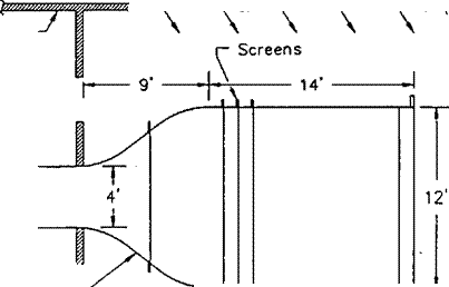
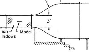
Fig. 2.1 Diagram of the Princeton University low speed wind Uinnel (not to scale).


image2image3image4

image5

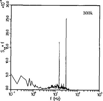
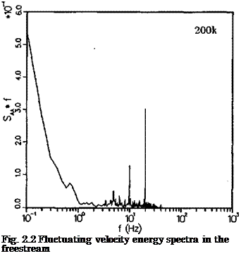
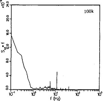
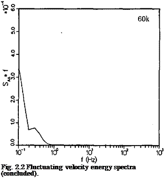
Подпись: Fig. 2.2 Fluctuating velocity energy spectra in the freestream

image7

Подпись:

image9

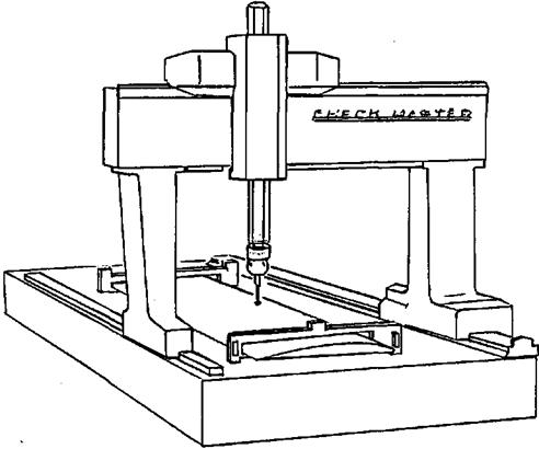
Fig. 2.3 Coordinate Measuring Machine (CMM) used for digitizing.

image10

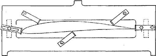
Fig. 2.4 Holding Fixture for digitizing the test sections.

37

31/1

XZ POINT

X= 13.6939 Z= -1.1266

38

32/1

X Z POINT

X= 13.7193 Z= -1.2182

! Upper L. E.

13

7/1

XZ POINT

X= 13.7199 Z= -0.7423

! Lower L. E.

15

9/1

XZ POINT

X= 13.6941 Z= -0.6770

Fig. 2.5 Typical CMM digitized data.

Подпись: AQUILA profiler data. Chord - 11.990 1.00000 0.00000 0.00106 0.99746 0.00123 0.00435 0.98829 0.00238 0.01274 0.97400 0.00453 0.05262 0.94486 0.00884 0.13491 0,90040 0.01570 0.24506 0.86567 0.02142 0.38540 0.83894 0.02575 0.53849 0.82217 0.02951 0.70417 0.80749 0.03199 ■ 0.79285 0.76590 0.03831 0.83603 0.69655 0.04901 0.88509 0.62461 0.06080 0.94190 0.54502 0.07190 0.97800 0.49234 0.07805 0.99740 0.39368 0.08685 1.00000 0.31264 0.08876 0.23528 0.08634 0.14185 0.07430 0.07922 0.05817 0.04595 0.04561 0.02491 0.03337 0.01583 0.02617 0.00659 0.01576 0.00169 0.00753 0.00000 -.00000 Fig. 2.6 Typical normalized coordinates from the digitized data.

Подпись: -.00259 -.00553 -.00714 -.00657 -.00665 -.00748 -.00767 -.00721 -.00651 -.00587 -.00546 -.00464 -.00375 -.00237 -.00083 0.00000

image11

. 2.7 Test rig indicating model orientation and lift measurement method. (Plexiglas end plates are not shown for clarity.)

image12

CLARK-Y-PT vs CLARK-Y (Althaus, 1980)

60.0 Подпись: о □ A Princeton

100.0 Princeton

200.0 Princeton

60.0 Model W. T. at Stuttgart

100.0 Model W. T. at Stuttgart

200.0 Model W. T. at Stuttgart

0.5

0.00 0.01 0.02 0.03 0.04 0.

-0.5 0.0

E374B-PT vs E374 (Althaus, 1985)

60.0 Princeton

100.0 Princeton

200.0 Princeton

60.0 Model W. T. at Stuttgart

100.0 Model W. T. at Stuttgart

200.0 Model W. T. at Stuttgart

Fig. 2.13 Comparison polars: E387A-PT vs NASA LTPT, Delft University, and Stuttgart.

E—387 data comparison for Rn = 200,000

G Princeton a NASA Langley LTPT 0 Low—Turbulence Tunnel at Delft v Model Wind Tunnel at Stuttgart

E—387 data comparison for Rn = 60,000

° Princeton

NASA Langley LTPT Low—Turbulence Tunnel at Delft Model Wind Tunnel at Stuttgart

FX60-100-PT vs FX60-100 (Althaus, 1980)

G 60,000 Princeton 0 100,000 Princeton A 200,000 Princeton s 60,000 Model W. T. at Stuttgart ® 100,000 Model W. T. at Stuttgart v 200,000 Model W. T. at Stuttgart

FX63-137B-PT vs FX63-137 (Mueller, 1985)

B 100,000 Princeton A 200,000 Princeton ш 100,000 Notre Dame

V 9ПП ODD Nntr#=> Пптр

0.00 0.01 0.02 0.03 0.04 0.05

Fig. 2.18 Comparison polars: NACA 0009-PT vs Stuttgart.

Force Measurement Technique and Instrumentation

Lift was measured directly using an electro-mechanical force balance, and the drag was found indirectly using the momentum method6. Rather than comput­ing the drag based on just one vertical survey, the wake was surveyed and the drag computed at four spanwise locations and then averaged.

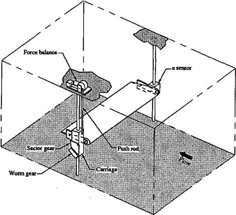
A sketch of the apparatus used to measure lift is shown in Fig. 2.7. The airfoil model was mounted horizontally in the tunnel between two | in clear plastic (Plexiglas) end plates (omitted for clarity) to isolate the model ends from the tunnel side-wall boundary layers and the support hardware. One side pivoted, and the other was free to move vertically on a precision ground shaft. Two linear ball bearings spaced 8 in apart provided essentially frictionless movement for a carriage which held the airfoil and angle of attack control hardware. Spherical bearings were used to minimize moments transmitted to each linear bearing. A force transducer coupled to the carriage through a pushrod sensed the lift (actually half the total model lift was transmitted to the transducer).

The force transducer in this study was a servo balance rather than a standard strain gauge or capacitance type transducer. As with a standard beam balance, the dead weight of the airfoil and the support structure are counterbalanced with weights. The remaining forces (the lift find residual imbalance) are balanced by the torque from a brushless DC torque motor mounted on the beam axis. Any angular displacement from a reference zero is sensed by an AC potentiometer, and the error signal is used to drive the torque motor until the error disappears. The torque required to do this is directly related to the lift. The current needed to generate the torque is a very linear analog of the torque, and therefore of the lift. ,

In practice several problems occur, the most difficult being to meet the re­quirement of low system friction. To achieve this, precision ball bearings were used throughout. The residual friction (as well as some magnetic hysteresis) was further reduced by adding a small amount of electrical dither to the torque motor. As built, the system was capable of measuring 7 lb (half of the lift) with stiction and hysteresis limited to 0.002 lb at the lowest Reynolds number. The overall system had an accuracy of ±0.25% of full scale or ± 0.002 lb, whichever is larger. The term full scale here refers to the maximum force experienced over a given run at constant Rn. This corresponds to ±0.0135 of Cj at Rn = 60k and ±0.0055 at 300k. Nine-point calibrations of the force balance were performed frequently to minimize the effects of drift.

The drag was measured using the momentum deficit method because the mechanical one is both difficult and expensive. In addition, drag obtained by mechanical means includes three-dimensional effects due to the side walls. These effects can be reduced by using a three-piece model with only the central panel connected to the force balance; however, the angle of attack of the two tips must be kept equal to that of the central portion and the gaps must be minimized. Althaus7 investigated the effect of a gap on the drag at low Rn and found that with a 0.5 mm (0.3%) gap and 250 mm (156%) span, the drag was increased 12% at an angle of attack of 9°.

To compute drag using the momentum method, a pitot tube was surveyed through the wake 1.25 chord lengths downstream of the trailing edge to find
the deficit. (Using a single pitot tube and moving it through the wake provided better spatial resolution of the wake than using a rake with multiple, fixed pitot tube locations.) Based on the application of the two-dimensional momentum and continuity equations to a control volume about the airfoil6, the drag force per unit span can be found as:

OO

Подпись: u(Voo — u)dyПодпись:d = p

— OO

where the integral is performed perpendicular to the freestream, downstream of the airfoil. The freestream velocity is Voo, у is in the direction normal to the freestream, and и is the x-component of velocity at the downstream location.

This method of determining the drag is valid only if the wake survey is made in a region where the static pressure is equal to that in the freestream. Surveys on several airfoils indicated that static pressures in the wake were nearly equal to the freestream static pressure.

For pitot tube misalignments of less than 10°, the measured total pressure is essentially independent of flow angle. The drag calculation requires only the streamwise component of the velocity; thus, transverse velocity components at the survey location can decrease the measured drag. Drag values were found to remain constant as the survey location was moved upstream and downstream of the 1.25 chord location, indicating that it was sufficiently far from the trailing edge so that transverse velocity components were negligible.

Drag was calculated using the difference between the total pressure upstream of the airfoil and that in the wake. Equation (l) can be rewritten to give:

OO ‘

d = 2 J (у/Pdoo – aj°o) {y/Pdoo – VPdoO ~ APo)dy (2)

— OO

where Pdoo is the freestream dynamic pressure measured with a pitot tube which was 15 in upstream of the airfoil and 8 in below the centerline, and ДР0 is the difference between the total pressure in the freestream and the total pressure in the wake. This pressure difference is small and difficult to measure, requiring a sensitive transducer. A Baratron model 220B unit made by MKS Instruments, Inc. was used for this purpose with a full-scale range of 1 mm Hg and am accuracy of 0.15% of reading. It was factory calibrated against a standard traceable to the National Bureau of Standards.

Spanwise non-uniformity in the wake is well known7,8. Indeed, the drag variation can be more than 50% at the lower Reynolds numbers. As mentioned previously, four spanwise stations spaced uniformly over the central 1 ft of the airfoil were used, and they were averaged to provide a better measure of the airfoil performance.

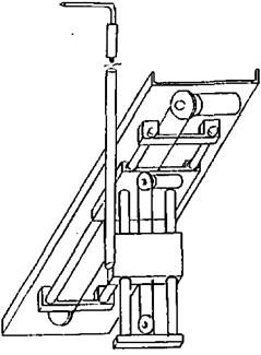
A two-axis traversing mechanism provided position control for the down­stream pitot tube (see Fig. 2.8). The important features and accuracies of this positioner are:

Spanwise motion: 24 in Vertical motion: 14 in Resolution:

less than 0.001 in, both directions Readout accuracy:

spanwise: 0.020 in vertical: 0.002 in Setability:

0.005 in, both directions

Each axis was instrumented with a precision DC potentiometer and was driven by a small, geared, DC motor. The carriage which held the pitot tube ran on precision bushings around centerless ground and polished rods, and the motors drove the carriage and potentiometers through a linkless steel and plastic chain. For stability, the entire carriage was mounted on a large aluminum “U” channel which was mounted to the bottom of the tunnel floor. The arm that carried the pitot tube projected into the tunnel through a slot cut in the floor, and both the arm and’slot were sealed to prevent air leakage into the tunnel.

Each motor and potentiometer together with associated electronics formed a position servo loop. The open-loop gain was quite high; however, the accuracy of the reading was independent of the gain, since it was read directly from the feedback potentiometers. Analog inputs to the positioner were provided by a computer with two digital-to-analog converters. Because accuracy was the design goal, there was no attempt to make the positioning particularly fast. This decision to ignore speed was soon regretted when it became apparent how long each run in the tunnel required. (Changes were made later that resulted in some improvement in the speed.)

Using this two-axis positioner, the surveys were made through the wake at four spanwise locations. Each survey consisted of between 20 and 80 pressure measurements (depending on the wake thickness) with points nominally spaced 0.08 in apart. A typical survey through the wake took two minutes, which effectively yielded a time-averaged drag value for each spanwise station.

Three pressure transducers (MKS model 220B) were used in this study. A 1 mm Hg full-scale unit measured the difference in total pressure between the wake and freestream as previously mentioned. Another 1 mm Hg unit measured the difference between the test section stagnation pressure and atmospheric pres­sure to allow an accurate calculation of the density in the test section. The third transducer had a 10 mm Hg full scale and was used to measure the dynamic pressure at the upstream pitot tube.

Due to the tunnel blockage from the lift apparatus installed in the test section, the velocity at the airfoil was greater than that upstream where the freestream dynamic pressure was measured. Since the upstream pitot-static probe did not sense the dynamic pressure at the airfoil, a calibration was performed to correct its reading. Using the continuity equation, it can be seen that the velocity ratio between the velocity at the airfoil and the velocity upstream of the blockage is simply the ratio of effective areas. Because the effective area of the apparatus is clearly a function of Reynolds number, a velocity ratio based on the Reynolds number was determined before every run. A velocity was found with the fixed upstream pitot-static probe and with the downstream pitot-static probe placed near the tunnel centerline with the airfoil installed but generating no lift. The ratio was determined at several speeds in the neighborhood of the actual run speed. A linear interpolation based on Reynolds number was then used during the run to determine the velocity at the airfoil based on the dynamic pressure of the upstream pitot-static probe. Throughout this work, the velocity difference between the upstream location and the airfoil was less than 6%.

During a run, which usually took about 1.7 hours, the tunnel velocity drifted slightly, depending on atmospheric conditions. To ensure ал accurate deter­mination of the lift and drag coefficients, the measured lift and the APq were normalized by the instantaneous value of the freestream dynamic pressure. Thus, slow fluctuations in tunnel speed affected only the Reynolds number and not the determination of the aerodynamic coefficients.

Wind-tunnel corrections6 were applied to values of C; and Cd and were ap­proximately 4% and 2%, respectively. Error estimates indicate that the accuracy of the measured Ci is ±1% and that of the Cd is ±4%. The angle of attack of the airfoil was controlled using a gear motor with a worm drive and a sector gear and was sensed using an angular transformer like that used in the force balance. The accuracy in determining a was ±0.02°.

All transducer voltages were recorded using a Scientific Solutions, Inc. 14-bit analog-to-digital converter interfaced to an IBM PC. The PC controlled the wake pitot tube position and the airfoil angle of attack. After manually setting the tunnel speed to achieve the desired Reynolds number, the data collection was completely automated and proceeded as follows: The first angle of attack was set, and the location of the wake was found. Next, the four wake surveys were performed. When they were complete, the angle of attack was increased and the process repeated. Usually, a polar at a given Reynolds number consisted of between 15 and 20 angles of attack from —3° to 15°. In all cases, this process continued into stall.

Drag was measured only for increasing angles of attack, so hysteresis was not examined. This was done for two reasons. First, the amount of run time would have doubled to 3.4 hours on average. Second, hysteresis is a sign of gross lami­nar separation—a high-drag condition. This investigation was directed towards the characteristics of low-drag airfoils in application to RC sailplanes; hence, high-drag conditions were of little interest. Furthermore, if the measured drag coefficient exceeded approximately 0.050 the run was stopped, again because there was no interest in high-drag conditions and also due to time constraints.

In addition to taking lift and drag data simultaneously, which was relatively slow, in many cases a second run was made in which just lift was measured, allowing the angle of attack to be incremented relatively rapidly. In this mode of operation, the angle of attack was increased up to a pre-set value and then decreased. Hysteresis loops present in the lift behavior were then sometimes observed. Approximately 140 data points were taken, and this process usually required 5 minutes—much less than the 3.4 hours that would have been required to obtain a complete drag polar at 1° increments in a. This lift data is included along with the polar data in Chapter 12. Increasing and decreasing angles of attack are denoted by solid-circle and open-square symbols, respectively. See Fig. 12.2 for example.

Digitizer Results

(Note, “-PT" (Princeton Tests) is appended to the airfoil name to distinguish the digitized coordinates from the nominal coordinates.)

In Chapters 10 and 11, each of the actual sections is plotted against the nominal coordinates at half scale (6 vs 12 in). The legend inside the airfoils shows what is being compared; the solid line is always the first airfoil, normally the prototype, and the broken line the second, normally the test section. In a few cases different prototypes are compared. Before they are plotted, the two airfoils are fitted in a least squares sense. The fitting uses two variables—relative vertical location of the entire section and relative rotation of the entire section— to produce the lowest possible RMS difference without distorting the airfoil. This difference is shown under the trailing edge of the upper plot.

The lower plot shows the difference, or error between the two airfoils on a much expanded scale. The upper surface difference is the solid line and the lower surface the broken one. If the two sections were perfectly matched, the plot would be two straight lines lying on the horizontal axis. A displacement above or below the axis means the test section surface lies above or below the nominal, respectively. If the solid line is above (or below) the broken one, regardless of its position with respect to the axis, the section is too thick (or thin) at that point. If both lines sweep up or down together then the camber is in error. Camber error as well as thickening is frequently seen at the trailing edge.

The short, inward-facing tics show the positions of the leading and trailing edges. The most difficult point to measure is the vertical position of the leading edge. (It is quite possible for a model to have more than one leading edge.) This is because the slope becomes infinite and a very small change in the chordwise position of the probe produces inordinately large changes in the measured thick­ness. Consequently, the vertical locations of the exact edges, as shown by the position of the tics, have somewhat reduced accuracy. However, because many points were digitized near the leading and trailing edges and because the contri­bution of each point to the overall accuracy number was weighted in proportion to the distance between it and the adjacent points, the effect of the end points on the overall error is very small. In addition, the most forward and most rearward points themselves were not included in the error calculation.

As a check on the digitizing procedure, two of the models were digitized more than once: the SD7080-PT and the SD7003-PT. The SD7080 pair was done early in the profiling as a general check for repeatability, but the spanwise stations were not the same. Even so, the agreement was within 0.003 in. The SD7003-PT was digitized six times; once at the beginning of the profiling, five times at the end (a time span of about 75 days). Two profiles, the SD7003-PT and SD7003-PT (R) were taken at the same station and are a good indication of the overall repeatability of the measurement setup—about 0.0007 in, 0.006% of chord. The remaining four profiles were taken at 3 in intervals centered on the span and were intended to discover how much spanwise variation a good airfoil model might show. As can be seen in Figs. 10.46-10.49, it is very small indeed.

Several observations can be made about methods of construction based upon the models digitized in this study. Built-up, sheeted models tended to have a problem with the blend between. the leading edge and the beginning of the sheeting. The trailing edge also tended to be thick. Foam core sections usually had sharper trailing edges, but any errors in contour were more prolonged; with built-up sections the errors were more local. One model had excellent contours for the separately molded upper and lower surfaces, except the joint at the leading edge was too wide. Because of the type of construction, the increased thickness at the leading edge carried back through a large part of the airfoil. This was a problem that was not present in models that used a single piece—usually wood—leading edge. The open-bay models have no single profile—over the ribs it can be accurate, but inevitably there is sag between the ribs.

Neither the cost nor the type of construction was a good indicator of the accuracy. For example, a balsa-sheeted, rib and spar section built over a weekend for under $10 had one of the most accurate profiles measured. On the other hand, the accuracy of some models costing many times this amount was only average.

Trailing edges are a problem for all types of construction. As can be seen from the plots, the most common error is a poorly contoured trailing edge; it is warped either up or down, with the preponderance being up. Since the

sensitivity of performance to trailing edge location is high, clearly there is a general problem here. One model, the S4180-PT, had a very thin trailing edge which was so warped that it was meaningless to measure it at all; there simply was no representative section. (This was the only model with such a major contour discrepancy.)

Some of the nominal airfoils differ less between themselves than the models do with the ideal coordinates. The HQ2/9, RG15, and S2048 are an example of this, and several plots compare these prototype sections. This has significance when comparing polars, because small differences in performance on similar sections could be a result of the inaccuracy of the model or random variations in the test results rather than an indication of the superiority of one prototype section over another. One model, the E193-PT, was actually a better fit to the E205 than to its true nominal coordinates (see Figs. 10.5 and 11.12). These airfoils are, of course, quite similar, but the point is that one must be careful in claiming performance for the prototype based on the model’s performance. In cases where the model is inaccurate, the performance applies to the model airfoil and not necessarily to the nominal airfoil.

One section, a SD7032, was first tested in the tunnel with no covering over the sanded balsa sheeting (version A: SD7032A-PT), then with Monokote covering (SD7032B-PT), and finally with a flap (SD7032C-PT). Only the flapped version was digitized.

The DF102-PT and DF103-PT are compared to the DF101-PT, not to a nominal airfoil. (The DF101-PT is compared to the nominal.) Since the point of these variants was to explore the effects of changes on the forward upper surface, the relevant prototype is the DF101-PT. The plots show what and how much was added or removed in that, area. The minor differences along the rest of the airfoil are due to the fact that the sample chords were not all at the same spanwise stations, and because the fitting routine tends to distribute the deliberate “error” over the entire airfoil so as to keep the RMS error down.

For a few airfoils (SPICA, WB135/35, and WB140/35/FB) the coordinates were supplied by the builders. In these cases small errors in fit are not meaningful because hand-generated coordinates are not smooth in the mathematical sense, and therefore the spline routine that compares the airfoils can have residuals of the order of the errors. This is particularly noticeable on the upper surface of the WB135/35 between 1% and 3% chord, where the model is smoother than the nominal.

Digitizing Procedure

The complete procedure from selecting the airfoil model to the end of the data reduction was standardized. The procedure was as follows: Since measurements

were generally taken at only one spanwise location, the airfoil was examined to be sure that this location was representative of the total section. If the covering had wrinkled, it was smoothed. Small, local distortions were excluded from measuring; however, larger distortions which covered most of the span, such as a flap joint or a long crack in the sheeting, were included.

The airfoil was held in two identical fixtures that supported the model in a level attitude on three points, see Fig. 2.4. These fixtures were designed so that when they were turned over the model was still supported on three points. Because of the impossibility of measuring both sides of the airfoil in a single position, machined reference blocks were permanently attached to the fixtures. These blocks could be touched by the probe with the fixture and model in either position (up or down). Consequently, when the section was turned over these blocks made it possible to maintain a single reference frame for both sides. The leading edge of the airfoil was aligned with one axis of the CMM table so the measured chord direction was perpendicular to the span, and so the same chord would be measured on both sides of the model. All the sections were of a constant chord so this point is not particularly important, but this method made it possible to check that nothing had moved during the measurements. (Because of the relatively non-rigid construction of the models compared to metal parts, the fixturing was free-standing on the machine’s table. There will be more on this later.)

As mentioned above, blocks mounted to the fixtures were used to establish the reference coordinate system for the upper surface. All points on the airfoil were referred by the software to the blocks, so the actual position of the airfoil and fixtures on the machine was unimportant. The chordwise location of the trailing edge was then determined by touching it with the probe from directly behind. This point was used to determine the actual chord of the section. Between 20 and 30 points were then touched on the upper surface. The spacing of points was more or less proportional to the local curvature; near the leading and trailing edges the spacing was small, over the central parts of the airfoil it was as great as ^ in. The final point touched in the upper surface sequence was the leading edge. This was detected by moving the probe vertically past it with the vernier lead screw at progressively closer settings until it touched.

Because of the possibility of distorting the model, the stands could not be rigidly held down to the CMM table. Consequently, any inadvertent movement during the data collection was detected by comparing the leading and trailing edge points as measured from both sides. If they were at the same points with respect to the reference frame established by the blocks on the fixtures, then no motion that could affect the measurement had occurred.

After the upper surface was done, the model and fixtures were turned over as a unit and the leading edge was once again aligned. Measuring continued at the leading edge, the first point here duplicating the last point on the upper surface, and the final point duplicating the first point on the upper surface (the trailing edge).

Of the 67 duplicated leading edge pairs, 46 were within 0.001 in, 52 within

0. 002, 59 within 0.003, 65 within 0.005 and all within 0.0057 in. Part of the difference within any pair is due to the impossibility of finding the exact point that was measured from the other orientation, because of the nature of the lead­ing edge. However, since a chordwise error translates to a much smaller vertical error except at the leading edge, these accuracies imply a general thickness mea­surement error of under 0.001 in. On a 12 in chord this is trivial.

The results of the measurements were collected on a Leading Edge personal computer, which was also used to reduce the data. All the output from the CMM was saved on a disk file. Typical output of the CMM software is shown in Fig. 2.5.

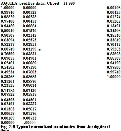
The CMM data are the locations of the center of the ball at the end of the probe, not the surface itself. Consequently, a second program was used to reduce the CMM output to the actual coordinates of the airfoil, to rotate the actual chord so it was parallel to the reference axis, and to normalize the airfoil to coordinates between 0 and 1. This data was also saved as a file. A header was added to identify the airfoil and show the actual chord. A typical output file from this program is shown in Fig. 2.6.

Wind Tunnel Models

In selecting the model size to obtain the desired Reynolds number, several tradeoffs were considered. To achieve a given test Reynolds number, the mea­sured forces increase with decreasing chord. While large forces are desirable, models with small chords are difficult to build accurately. For this work, a model shop was not used; rather, experienced model sailplane enthusiasts were solicited to build the models. Consequently, construction tolerances were on the order of that found on model sailplanes. For these reasons a 12 in chord was selected as a compromise between the two competing effects. The model span was 33 I in. Construction techniques ranged from all-balsa with ribs, spars and open bays, to fiberglass-covered foam. All models were fully-sheeted except one, which had open-bay construction (see NACA 6409).

2.2.1 Digitized Profiles

As a check for model accuracy and for later airfoil performance computa­tions, every model was profiled using a digitizing Coordinate Measuring Ma­chine (CMM) to obtain the actual airfoil shape. A comparison was then made with the desired airfoil shape to determine the accuracy of the model. Profiling was performed at Fraser-Volpe Corporation in Warminster Pennsylvania using a Helmel Checkmaster CMM with full computer software for measurement pro­cessing. This machine and software made it possible to determine the location of a point in space within 0.0005 in absolute and 0.0003 in typical for all three axes.

A drawing of the CMM is shown in Fig. 2.3. The machine itself consists of a marble slab which is finished to a high surface flatness. On the slab is a gantry which can traverse the length of the table. Mounted on this gantry is a second gantry which in turn holds a vertical column to which the probe is attached. This arrangement allows the probe to be positioned anywhere within a large volume beginning at the surface of the slab. The probe consists of a hard plastic ball mounted to the end of a steel shaft which is screwed into a precision motion detector. The equivalent measuring diameter of a probe is found (the probe is said to be “qualified”) by touching it to a sphere of precisely known diameter. The computer then calculates the measuring diameter using basic geometry. Coordinates are read from the sensors when the probe is deflected in any direction by approximately 0.0003 in from its rest position. (This deflection is automatically accounted for by the CMM software.)

Outputs from the three sensors are routed to a computer which runs com­mercial software allowing one to reduce the raw information from the three axes to determine diameters, lengths, angles, differential locations, rotations, many different kinds of deviations from standard shapes, and so on. It will refer all measurements either to the table itself or to an arbitrary coordinate system based on the part or its fixtures. Indeed, setting up this coordinate system, or reference frame as it is called, is a major part of any measurement.

In addition to simply making a measurement, the computer can be “taught” a program of steps which represent a specific series of measurements. The com­puter will then prompt the operator for what point to measure next, and “knows” what to do with the measurement once it is taken. This capability was used here, allowing the entire process of measuring a model to be completed in about 25 minutes, including fixturing and post-measurement data reduction.

The machine is routinely calibrated to standards traceable to the National Bureau of Standards.