Many critical tasks performed hy pilots involve them in activities that resemble those of a servo control system. For example, the execution of a landing approach through turbulent air requires the pilot to monitor the aircraft’s altitude, position, attitude, and airspeed and to maintain these variables near their desired values through the actuation of the control system. It has been found in this type of control situation that the pilot
492 Dynamics of atmospheric flight Table 12.3
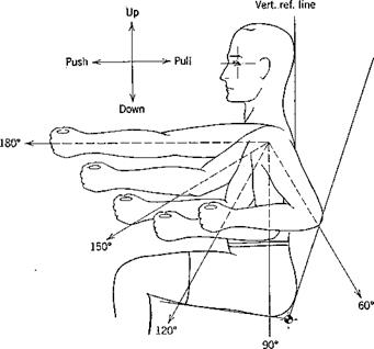
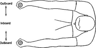
Hand-Operated Control Forces (From Flight Safety Foundation Human Engineering Bulletin 56-5H) (see figure on page 495)
|
Direction of Movement
|
180°
|
150°
|
120°
|
90°
|
60°
|
Values given represent maximum exertable force in pounds by the 5 percentile man
|
|
Pull
|
Rt. hand
|
52
|
56
|
42
|
37
|
24
|
|
Lift, hand
|
50
|
42
|
34
|
32
|
26
|
|
Push
|
Rt. hand
|
50
|
42
|
36
|
36
|
34
|
|
Lft. hand
|
42
|
30
|
26
|
22
|
22
|
|
Up
|
Rt. hand
|
14
|
18
|
24
|
20
|
20
|
|
Lft. hand
|
9
|
15
|
17
|
17
|
15
|
|
Down
|
Rt. hand
|
17
|
20
|
26
|
26
|
20
|
|
Lft. hand
|
13
|
18
|
21
|
21
|
18
|
|
Outboard
|
Rt. hand
|
14
|
15
|
15
|
16
|
17
|
|
Lft. hand
|
8
|
8
|
10
|
10
|
12
|
|
Inboard
|
Rt. hand
|
20
|
20
|
22
|
18
|
20
|
|
Lft. hand
|
13
|
15
|
20
|
16
|
17
|
|
Note: The above results are those obtained from unrestricted movement of the subject. Any force required to overcome garment restriction would reduce the effective forces by the same amount.
|
can be modeled by a set of constant-coefficient linear differential equations (termed “human-pilot describing functions”). Much of the original research in the field of human-pilot describing functions has concentrated on the pilot’s performance in a single degree of freedom compensatory tracking task with random-appearing system inputs. In a single-degree-of-freedom task the pilot controls a single state variable through the actuation of a single control. A compensatory display is one in which the tracking error is presented, regardless of the source of the error. Fig. 12.1 shows the block diagram for such a task. Here a pilot is concentrating on controlling the pitch attitude
|
Turbulent air disturbance

Fig. 12.1 Typical compensatory task.
|
of the aircraft through the use of the artificial horizon display. The system input in this case is turbulent air which produces random pitching motion of the vehicle.
The pilot model used in compensatory tasks consists of the describing function and the remnant as shown in Pig. 12.2. (See also Sec. 3.5.) Here the task is the same one presented in Fig. 12.1, but the human pilot has been replaced by a mathematical model. The model consists of two parts, as shown: Y(s), the linear describing function (written in Laplace transform notation), and n(t) the remnant. Since a linear model is never able to describe the pilot completely, Y(s) is insufficient by itself, and it is necessary to include the remnant n(t), which is that signal that must be added in order to have all the time signals circulating in the system of Fig. 12.2 correspond exactly to those of Fig. 12.1 when the identical input is present. The Y(s) selected to describe the pilot in any particular task is chosen so as to minimize that part of the input signal to the aircraft which arises from n(t). Thus the linear pilot model that results is that which accounts for as much pilot input to the aircraft as possible, and a measure of its adequacy is the fraction of the pilot input to the aircraft accounted for by Y(s).
|
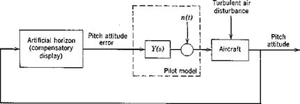
Fig. 12.2 Compensatory task with pilot model.
|
The human-pilot describing function is useful in studying two classes of problems. In the first the describing functions derived from previous research are utilized to aid the systems designer. With a mathematical description of the pilot at hand he can close the loop around the mathematical description of the proposed vehicle in order to predict the overall system response. The second type of study involves the measurement of actual human-pilot describing functions as the pilot flies a particular vehicle in order to obtain an objective measure of how the task affects the pilot.
Due to the complex nature of the situation it is possible to model the pilot in many ways and to measure the model by employing a variety of techniques. One of the most successful approaches to the measurement problem utilizes power-spectral-density measurements of signals circulating in the control loop. The general case of a tracking task of one degree of freedom with a compensatory display is illustrated in Fig. 12.3a. In this task the pilot must control the aircraft response m(t) in such a fashion that it matches as closely as possible the desired aircraft response i(t). The pilot does this by viewing the instantaneous error e(t) and altering his input o(t) to the aircraft. It is found that the pilot’s control technique is primarily influenced by the type of input i(t), the dynamics of the control system, the type of display and the dynamics of the aircraft. Any useful pilot model must reflect these influences.
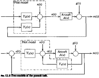
Past research in this field has concentrated on tasks with random appearing input signals i(t) because so many real-world situations involve this type of disturbance. Thus the pilot models that have been developed apply strictly only to tasks with the above type of input. The system of Fig. 12.3a is modeled by that of Fig. 12.36. Note that the model includes the dynamics of the control system and that the signal o(t) corresponds to the position of the control column. It has been found that in the frequency band of primary interest and for the type of controls normally found in aircraft, such a model is fairly insensitive to the exact control system used and that pilot models developed on this basis are quite general. Now the linear system of Fig. 12.36 can be redrawn as the point by point sum of the two linear systems of Fig. 12.4 (if the aircraft is assumed to be a linear system). It follows that
e(t) = eft) + eft)
o{t) = off) + oft)
m(t) = mft) + m2(t)
The describing function Y(s) is chosen to minimize the r. m.s. value of oft). Note that this is not the same criterion as used in defining the open-loop describing function in Sec. 3.5, where the mean-square-remnant was minimized in the presence of a fixed input. The difference of course is that we are dealing here with a closed-loop system, in which signals derived from the remnant circulate the loop and appear at the input to the pilot. The process of minimizing o22(t) can he carried out in a manner basically similar to that used in Sec. 3.5 with the result (ref. 12.2)
Y(ico) = Фі0(а>)ІФіе(а>) (12.2,1)
where Фг0(<ы) is the cross-spectral density of i(t) and o(t) etc. (See Sec. 2.6). We also find that Фіп(т) = 0,—i. e. the remnant is uncorrelated with the input signal i(t). This linear model, T(-s), is a best fit in the root-mean-square
|
DIRECTION OF MOVEMENT
|
 |
|
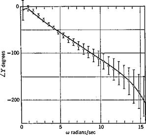
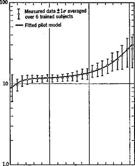
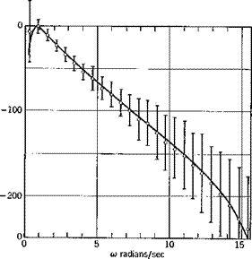
Fig. 12.5 Experimentally measured pilot model, compensatory display, (from ref. 12.5)
|
|
|
|
|
~l I I I j I I I I Bandwidth of i(f)-2.8 rad/sec Aircraft dynamics-if/s
|
|
 |
This form is preferred for measurement because it is not possible to measure o2(t) directly. The remnant n(t) exists because in actuality the human pilot is not operating exactly as a linear/invariant mathematical system. The signal n(t) is a random-appearing variable and hence is not predictable. However, some measurements have been made of its statistical properties (ref. 12.6) over a range of task variables. Figure 12.5 shows a typical experimentally measured pilot describing function together with p2. In this task the input to the pilot was the deflection of the artificial horizoil display (in inches) and his output was control column deflection (in degrees). It is seen from the plot of p2 that the describing function models the low-frequency performance of the pilots quite well, but is less satisfactory for a> > 5 rad/sec.
 |
 |
The following form for the describing function has been developed to cover the single-degree-of-freedom compensatory tracking task with a random-appearing input (ref. 12.3):
(12.2,2)
In this formulation e~TS represents the pure transmission time delay within the pilot associated with nerve conduction and stimulation, т is estimated to range from.06 to.10 sec. The factor in curly brackets is a reasonable representation of the dynamics of the neuromuscular system of the arm with typical values: 1/TN = 10 sec-1, ojn = 16.5 rad/sec, and £jV = .12. (TKs + 1)/(T’Ks – j – 1) represents a very low frequency lag-lead component. The remaining terms Kp[(TLs – f 1)I(TjS -j – 1)] are the adaptive portions of the model; the values of Kv, TL, and Tj are altered by the pilot to suit the particular system being controlled. It is found that for most engineering applications, in which an exact pilot model is not required at very low and very high frequencies, an adequate approximation is

 {TLs + 1)
{T f + 1 )(2> + 1)
The following set of adjustment rules for the pilot model have been developed by McRuer et al. (ref. 12.3).
1. Stability: The human adopts a model form to achieve stable control— i. e. one that produces a stable closed-loop system.
2. Form selection—Low frequency: The human adopts a model form to achieve good low-frequency closed-loop system response to the input signal. A low-frequency lag, Tz, is generated when both of the following conditions apply:
(a) The lag would improve the low-frequency characteristics of the system.
(b) The aircraft dynamics are such that the introduction of the low- frequency lag will not result in destabilizing effects at higher frequencies that cannot be overcome by a single first-order lead, TL, of somewhat indefinite but modest size.
3. Form selection—Lead: After good low-frequency characteristics are assured, within the above conditions, lead is generated when the aircraft dynamics together with the pilot time delay are such that a lead term would be essential to retain or improve high-frequency system performance.
4. Parameter adjustment: After adoption of the model form, the describing
function parameters are adjusted so that:
(a) Closed-loop low-frequency performance in operating on the input signal is optimum in some sense analogous to that of minimum mean-squared tracking error.
(b) System phase margin, фм (see Sec. 11.6), is directly proportional to а>{, the input signal bandwidth (loosely defined as the frequency above which the input spectrum decreases rapidly), for values of ojj less than about 2.0 rad/sec. The strong effect of forcing-function bandwidth on the phase margin is associated with the variation of TN with со{.
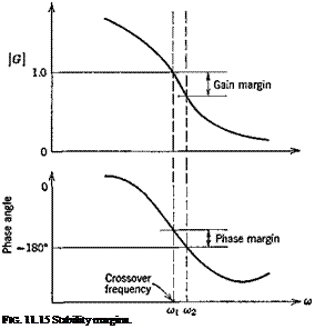
. (c) Equalization time constants TL or Tp. when form selection requires 1 jTL or 1 jTj << a>c, the system crossover frequency (the frequency at which G(ico) H(ico) equals unity—see Eig. 11.15), it will be adjusted such that low-frequency response will be essentially insensitive to slight changes in TL or Tx (for co{ << oof).
5. ooc Invariance properties:
(a) Independence of coc w. r.t. Kc: Let the aircraft static gain be Kc, and that of the pilot be Kv [see (3.2,4) and (3.4,26)]. After initial adjustment, changes in Kc are offset by changes in the pilot gain, Kp; i. e. system crossover frequency, coc, is invariant with Kc.
(b) Independence of coe w. r.t. co{: System crossover frequency depends only slightly on the input bandwidth for ші < 0.8caco. (coeo is that value of u)c adopted for ooi « coe.)
(c) ct)c Regression: When oji nears or becomes greater than 0.8coco, the crossover frequency reduces to values much lower than ooco.
Although the above pilot model was developed to describe the single – degree-of-freedom compensatory tracking task, it is finding more and more use in the general situation of the multiple-loop tracking task. In such a task the pilot controls a number of vehicle variables simultaneously. It has been found that the same basic form of pilot model can be applied in many cases with slight modification to the values of some of the parameters (such as the time delay t) to account for the additional complexities of the task (such as visually sampling the outputs of several instruments). In this application a single describing function is used to close each control loop actually closed by the pilot. For example, if the task is to control both the pitch and roll attitudes (assuming the pitch and roll modes to be uncoupled), one describing function would close the roll loop while a second would close the pitch loop.


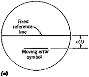
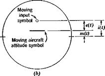 Fig. 12.6 Displays, (a) Compensatory. (6) Pursuit.
 Ф0»
Ф0»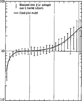




 {TLs + 1)