Category Management and Minimisation of Uncertainties and Errors in Numerical Aerodynamics

Development of the Sensors

In order to quantifly and handle the errors and uncertainties arising, sensors for their detection were developed and implemented. These sensors scan the boundary layer and flow field to ascertain the level of adherence to relevant best practice guidelines. These sensors are developed and calibrated on the basis of a generic test case using a reference solution with minimal error. A sensitivity study with isolated mechanisms was carried out first of all, following which the interaction of errors was investigated for mixed errors. The results were parameterized to give simple expressions for the error magnitude as a function of the relevant sensor output. The applicability of these derived functions to more complex test cases is tested.

1.1 Development of the Error Sensors

At the beginning of the investigation the grid convergence study was performed on the flat plate test case (Re = 2.1e6, Ma = 0.1, u0 = 33m/s) with a fully structured grid. For this the turbulence model of Spalart-Allmaras with Edward-modification (SAE) was used, which is the specified standard model in TAU. The grid expansion ratio near the wall and the wall distance y0 of the wall nearest grid point were varied until there were no significant changes in the solution. The hereby identified grid was used as a reference grid and as a basis for the further investigations. For all investigations eight different turbulence models were applied — two one-equations models (SAE and Spalart-Allmaras (SAO)), three two-equation models (Wilcox k – ю, Menter-SST und LEA к-ю) and three EARSM models (Rung RQEVM, Wallin & Johannson 2D Mean Flows (WJ2D) und Hellsten EARSM к-ю).

Classification of Errors and Uncertainties

The structuring of this work is based upon the distinction between errors and uncer­tainties, for which the definitions given in the BPG for industrial CFD published by ERCOFTAC [1] are adopted.

Errors

The term error is used to refer to problems arising from mis-use of the flow solver or turbulence model and is distinct from the functionality of the applied model. Errors hence lead to different predictions for the same flow using the same model and a prominent example is the use of an insufficiently fine grid. Errors can in theory be avoided through proper solution setup (i. e. by an experienced user and/or through adherence to an appropriate set of BPG). Nonetheless, the problem of errors should not be under-estimated since they are often hard to identify and to avoid, particularly in complex industrial configurations. Furthermore, advanced knowledge of the flow solution is required to correctly generate the grid. Examples include the choice of the skin friction normalised wall-normal cell size at solid boundaries, y+, the wall – normal expansion ratio of the grid inside the boundary layer, the recommendation of wall-normal grid cells and the capturing of the complete boundary layer with prismatic cells.

Uncertainties

In contrast to errors, the term uncertainty is used to refer to loss of predictive ac­curacy that occurs due to lack of knowledge about the true flow physics. In the scope of this work, this implies shortcomings of the RANS models in describing the turbulence. Deviation of an error-free solution with “reality” can hence arise due to uncertainties. The varying reliability of different turbulence models for dif­ferent flow phenomena, e. g. separating/reattaching flows and shock-boundary layer interaction, is primarily considered. Compared to errors, BPG concerning RANS modelling uncertainties are more vague in nature and less accessible to a “Boolean” type of treatment: Simple statements along the lines of “Model A is best for flow type X” have remained elusive.

Minimization and Quantification of Errors and Uncertainties in RANS Modeling

Tobias Schmidt, Charles Mockett, and Frank Thiele

1 Introduction

Owing to their affordable computational cost relative to higher-fidelity approaches such as large-eddy simulation (LES), statistical turbulence models are currently the principle workhorse for the simulation of turbulent flows in industrial aerodynamics. However, significant problems arise from the inherent empricism of such Reynolds – averaged Navier-Stokes (RANS) approaches. First and foremost, the current state of the art is that no universally-applicable model is available. Instead, a very large number of different RANS models exist, with varying degrees of mathematical com­plexity and with calibration valid for limited classes of flows. This state of affairs is further compounded by the experience that more complex formulations do not necessarily deliver better results. For these reasons, the choice of turbulence model for an engineering simulation has a strong impact on the quality of the results ob­tained. In addition to this, simulation results using a fixed RANS model show a strong sensitivity to other aspects of the simulation setup, most notably the grid. For external aerodynamics applications, the spatial resolution of the thin boundary layer regions is seen to be particularly important. All these factors lead to a very high dependency on the decisions made by the engineer in setting up the simulation, and strong reliance is placed on a combination of best practice guidelines (BPG) and user experience.

The motivation of this work is therefore the development of a series of extensions to the TAU flow solver, intended to reduce this user burden and to improve the quality of simulation results in an industrial environment. The approach taken is the development of a range of sensors to check important grid design parameters

Tobias Schmidt • Charles Mockett • Frank Thiele TU Berlin, Muller-Breslau-Str. 8, D-10623 Berlin

e-mail: {tobias. schmidt, charles. mockett}@cfd. tu-berlin. de, frank. thiele@cfd. tu-berlin. de

B. Eisfeld et al. (Eds.): Management & Minimisation of Uncert. & Errors, NNFM 122, pp. 77-100. DOI: 10.1007/978-3-642-36185-2_4 © Springer-Verlag Berlin Heidelberg 2013

and to detect the occurrence of flow phenomena known to be correlated with high model-dependency. For the grid error sensors, this amounts to the incorporation of BPG within the software itself. With these sensors in place, the next step is to attempt to quantify the error introduced. For this, the feasibility of an empirical approach is assessed, whereby the solution sensitivity to various error mechanisms is established on simple datum test cases and extrapolated to more complex flows. The implemented module provides the engineer with enhanced textual and graphical feedback, drawing attention to possible problems and suggesting appropriate steps to improve results and minimise such errors.

Conclusion

The methods of adjoint error estimates and local mesh modification are applied to several test cases. The main focus was set on the global aerodynamic coefficients. Only for the mesh repairing the focus was set on the validity and the computablility of meshes.

For the adaptation series of the DLR-F6 with the adjoint error estimates no final conclusion can be given. The numerical values given by [12] are widely spread. The corresponding experimental data show for some coefficients improvements and for some not. At least one should note that a comparison of the experimental results for Re = 3 • 106 measured in the NASA NTF and in the ONERA S2MA facility shows as well differences especially in the drag [7]. If one projected these differences to the measurements at Re = 5 • 106 the adapted meshes would show an improvement for all coefficients.

However, the results of the adaptation series converge for both used sensors to similar values which are different from the values of the finest mesh. The results on the meshes which are locally modified to satisfy a quality measure based on an anisotropic metric are close to the results computed on the original meshes.

For the high-lift configuration the adjoint approach improves the results in the linear region of the polar. The values of maximal lift are ambiguous and depend on the used meshes. The deviations of the results on the meshes which are optimized to

(b)


(c)


Conclusion

ConclusionConclusionConclusion

Conclusion

Conclusion

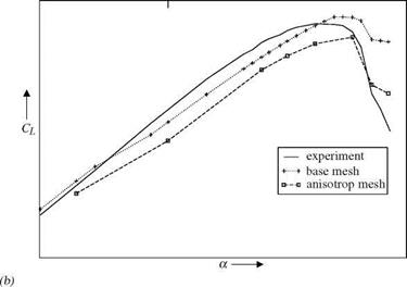
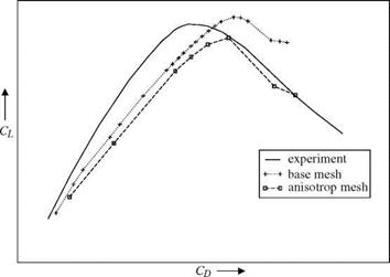
Fig. 13 (a) Lift Cl as function of the angle of attack a for the TC-217 model. (b) Polar for Cl and Cd of the TC-217 model. + marks the results computed on the base mesh. □ denotes the results on the modified meshes. The solid line shows the experimental results.

an anisotropic quality measure increase. The reason for the strong deviations have to be analyzed.

The results for the adjoint approach show additionally that the strategy to use one grid for the whole polar works even if the adaptation was performed only for a specific angle of attack. This strategy reduces significantly the computational effort and makes the adjoint approach applicable.

The repairing of meshes was successfully demonstrated for several meshes. This method is useful if a computation on a mesh due to numerical errors or negative elements fails and a new mesh generation is not desirable.

3 Outlook

[13] couples the adjoint adaptation with the feature of anisotropy. He demonstrated that with this mixed approach the convergence of the coefficients is much faster than with an isotropic mesh adaptation. [13] states that the adjoint approach balances the inaccuracies which can occur by the anisotropic meshes and uses the positive effects of anisotropic meshes. This has to be tested with the present methods.

Additionally the introduced error estimation approach of [2] tries to reduce the error with respect to numerical dissipation terms. The original work of [13] tries to reduce the error with respect to the discretization itself. A comparison of both approaches would also be interesting.

Acknowledgements. The author is grateful to R. Heinrich and E. Elsholz for providing the shown test cases for the mesh repairing.

Mesh Modification with Anisotropic Quality Measures

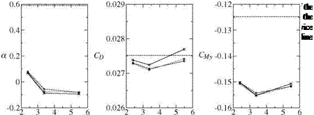
The mesh modification was applied to the DLR-F6 test case described in sec­tion 3.1.1 to see the influences on the aerodynamic coefficients. Again a target lift computation for CL = 0.5 was performed. After the flow computation the coarse, medium and fine mesh was modified by using a quality measure which uses an an­isotropic metric. The metric was derived from the Hessian of the local Mach number. The flow was recomputed on the anisotropic mesh. This procedure was performed twice.

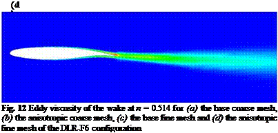
In figures 11(a)-(c) the angle of attack, the drag and the pitching moment are plotted as function of the grid points NP. The results computed on the base meshes are denoted by x. The results of the first and second mesh modification step is marked by о and □. The major improvements are observable for the drag on the coarse mesh, but the differences to the original mesh are relatively small in comparison to the changes caused by an adaptation with the new sensors. The major changes are observable in the resolution of the wake. In figure 12 the eddy viscosity is shown on four different meshes. The eddy viscosity on the coarse and fine base meshes (figure 12a,c) dissipates in the unstructured part very quickly, where on the anisotropically modified meshes (figure 12b,d) the wake is more resolved behind the wing, even on the coarse mesh. The improved wake resolution is observerable on the whole configuration.

In a second test the mesh modification with an anisotropic quality measure was applied to the TC-217 configuration (see section 3.1.2). For the test the mesh modi­fication with the anisotropic quality measure was applied twice to the base mesh for а = «1. Again the metric was derived from the Hessian of the local Mach number. The results are presented in figure 13. The + and □ denote the results on the original and the modified mesh, respectively. Due to the mesh modification the lift decreases

Mesh Modification with Anisotropic Quality Measures
by 8Cl « 8LC. The drag increases by SCd ~ 100DC. The result on the modified mesh increases the differences to the experimental results.

Mesh Manipulation

2.3.1 Repairing of Meshes

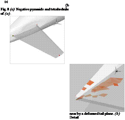
Negative elements occur many times by applying a deformation on the mesh, e. g. for CFD/CSM coupling. The appearance of negative cells permits a CFD compu­tation on those grids. To avoid a new meshing of the deformed geometry and to measure effects below the uncertainties of mesh effects the negative cells have to be repaired. Here the repairing of negative elements was successfully demonstrated on two configurations. An isotropic metric was chosen to calculate the quality measure.

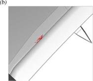
The first test case was a clean wing/body configuration with horizontal tail planes. To trim the configuration the horizontal tail plane was deformed. Due to deformation of the tail plane 83 elements with a negative volume occur (figure 8). These inverted elements are tetrahedrons and pyramids. By applying the mesh modi­fication all negative elements vanish.

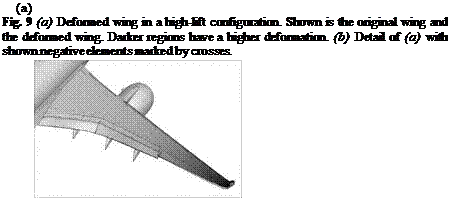
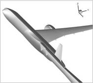
The second test case was a commercial aircraft including wing, body, nacelle, pylon, vertical tail plane and flap track fairings in a high-lift configuration (fig­ure 9a). Due to the applied deformation, 26 tetrahedrons have a negative volume. These elements are located in the slot between the flap inboards and the wing (fig­ure 9b). Again, by applying the implemented mesh modification all negative tetra­hedrons are inverted to valid elements with a positive volume.

In many cases the generation of negative elements can also be prevented by ap­plying the mesh modification on elements with a low quality before the mesh is deformed. For example in the previous case of trimming the horizontal tail plane, negative elements were prevented if the mesh was improved before the deformation step is performed.

Mesh Manipulation

Mesh Manipulation

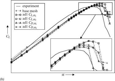
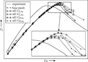
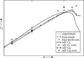
Fig. 7 (a) Lift Cl as function of the angle of attack a for the TC-217 model. (b) Polar for Cl and Cd of the TC-217 model. + marks the results computed on the base mesh. о and □ denote the results of the meshes adapted with the adjoint lift sensor for a1 and a2. Д and x show the results for the adapted grids with respect to the drag. The solid line shows the experimental results.

Mesh Manipulation
Mesh Manipulation
Mesh Manipulation

Another application of the mesh modification is the improvement of the quality of the unstructured part of the mesh when the computation on the mesh diverges. In figure 10(a) an example is shown where many tetrahedrons have a bad shape. By applying the mesh modifications the number of badly shaped elements decreases significantly (figure 10b). The number of tetraherons with a dihedral angle less than one degree decreases from N^<1o = 6840 to N^<1o = 29. The number of tetraherons with a dihedral angle less than five degree decreases fromN^<1o = 34598 to N^<1o = 252. Note that after the improvement of the mesh a converged CFD solution could be achieved.

Mesh Manipulation Mesh Manipulation

Fig. 10 Mesh with many badly shaped tetrahedral elements before (a) and after (b) the mesh modification. In both figures elements with a dihedral angle less than one degree are shown.

TC 217

The adaptation sensor based on an adjoint error estimate is also applied to the second test case of the TC 217 high-lift configuration. The model was a wing/body configur­ation with deployed slat and flaps. The geometry was previously used in the EURO­LIFT project. The flow parameters are Ma « 0.18, Re « 1.5 • 107 and Tref « 114°K. All computations are performed with the Spalart-Allmaras turbulence model.

For this configuration the polar was computed on a mesh with NP = 10733766 grid points. Outgoing from this mesh for several angles of attack an adaptation with the new sensor (4) was performed. Like for the DLR-F6 model the adaptation was repeated several times. The number of points increases within each adaptation step by 30%. In contrast to the DLR-F6 test case convergence problems occur on this configuration, e. g. the convergence was too slow and the computational effort too high or the adjoint computation diverges. However, for most of the angles of attack one adaptation iteration was successfully performed. In figure 6 the results of this first test were plotted. The + shows the result of the computation on the base mesh. The corresponding experimental values were plotted as solid line. The major differ­ences are observable in the linear region and near the maximal value of lift CLmax.

ai a2

TC 217

Fig. 6 Lift Cl as function of the angle of attack a for the TC-217 model. + and о denote the results on the base mesh and the corrected values by the adjoint error estimation, respectively. x and * mark the results of the first adaptation step with a sensor based on lift and drag, respectively. The Д and 0 are the corrected values. The solid line denotes the experimental results.

For lower angles of attack the computational results have a step-like shape. On the other side of the curve the angle of attack and the corresponding lift is too high. The values of the lift corrected by the adjoint error estimate (□ in figure 6) are higher then the original ones.

Outgoing from these results the mesh was adapted for several angles of attack a with the adjoint error estimate for lift (x in figure 6) and drag (* in figure 6), respectively. For both sensors an improvement of the linear region is observable. The step like behaviour vanishes. In the nonlinear region the results (if they are available) are similar to the results on the base mesh. The corrected values for the adapted grids are higher than the original values. Unfortunately most of the adjoint computations fail. Due to this experiment and the high computational effort four adapted meshes are selected from the linear and the nonlinear region. The four selected meshes are the meshes adapted by the lift or drag sensor for a = a1 and a = a2 (see figure 6), respectively. The results are plotted in figure 7. The results on the base mesh are marked by +. The results of the lift adapted mesh at a1 and a2 are denoted by о and □, respectively. The results of the drag adapted meshes are denoted by Д and x.

In figure 7(a) the lift is plotted as function of the angle of attack. In the linear region the values on the adapted meshes are close together. The deviation between the meshes ad1 CL, a1 and ad1 CDa1 is SCl « 1LC. The offset between the meshes ad1 Cl, a2 and ad1 Cd, a2 is of the same order. The offset between the adapted meshes and the base mesh is about SCl « 10LC for a < a1. The step like behaviour in the lift curve at a « a1 vanishes due to the adaptation. In the nonlinear region close to maximal lift the results of the adapted meshes diverge from each other. The results on the meshes which are adapted at a2 show a higher maximal lift coefficient (8Cl ~ 3LC with respect to the base mesh) and also the angle of attack of maximal lift is shifted by 8a « 1° relative to the results on the base mesh. The maximal lift value on the meshes adapted in the linear region at a1 have a lower value than the lift on the base mesh. The offset in the position of the maximal lift is 8a « 0.5°.
In figure 7(b) the lift is plotted as function of the drag. Again the results on the adapted meshes are close together in the linear region. At maximum lift the results on the meshes adapted at ai diverge from the values of the meshes adapted at a2.

All computations differ from the experimental results. The slope of CL(a) is lower for the computational results than in the experiment. The values of maximal lift are higher than in the experiment. The same holds for Cl (Cd ) in figure 7(b). However, in the linear range an improvement by the new method is observable due to the vanishing of the step like behaviour in the linear region. The improvements for the maximal lift are ambiguous.

DLR-F6

This test case was defined for the Third AIAA CFD Drag Prediction Workshop [see 12]. The flow parameters for the DLR-F6 wing/body configuration are Ma « 0.75, Re « 5 • 106 and Tref = 322.22. The meshes were taken from the workshop[1].

The first test on this configuration is a comparison of a mesh refinement study and an adaptation series with the new sensors. For the refinement study a computation on a coarse (NP = 2464385), a medium (NP = 5102446) and a fine (NP = 8535263) mesh was performed. For all computations the lift is targeted to Cl = 0.5 and the Spalart-Allmaras turbulence model was used. Outgoing from the coarse mesh the adaptation was repeated five times with the new sensor given in equation (4). The number of points increases within each adaptation step by 30%. Additional to the flow computation in each adaptation step the adjoint error estimation was computed.

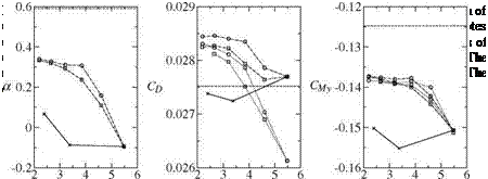
The values of the angle of attack a, the drag Cd and the pitching moment CMy of the refinement study are plotted in figure 3(a)-(c) as function of NP 2/3. The crosses show the results of the coarse, medium and fine mesh. The circles and squares con­nected by solid lines are showing the results of the adaptation with the new sensors for lift and drag, respectively. Signs connected by dotted lines denote values which are corrected by the adjoint error estimate (3). The results from the refined meshes show an ambiguous behaviour regarding the convergence for all plotted coefficients. In contrast the results from the adaptation series converge approximately to distinct values. The corrections by the adjoint error estimate decrease continuously so that finally the corrected values converge to the uncorrected values. The values of the finest meshes of the adaptation series are higher than the values from the finest mesh, e. g. ACd ~ 10DC.

A comparison with the results given in [12] shows that the results of the refined and of the adapted meshes are lying in the range of other codes. Additionally [12] make a statistical analysis of the values for drag. Their estimate for the mean of the drag is Cd = 0.0269, the standard deviation is о = 0.0006. Here the values of the adaptation are significantly out of this range.

The experimental results are taken from [7]. The measured values are shown in figure 3(a)-(c) by a dashed line. For the angle of attack and the pitching moment the adapted grids are lying closer to these experimental results than the results of the refined meshes. For the drag the values on the refined meshes are closer to the experiment.

In the second test a polar is computed. Again the flow conditions are Ma « 0.75, Re « 5 • 106 and Tref = 322.22°K. Instead of a fixed target lift coefficient here the angle of attack was varied in the range of a = [-5°, 2°]. The polar is computed on

DLR-F6
the coarse, medium and fine mesh. To avoid the computation of an adjoint solution for each angle of attack, four adapted meshes from the previous adaptation series for lift and drag are used. Here the mesh from the first (ad1) and the third adaptation (ad3) step with NP « 3.2 • 106 and NP « 5.5 • 106 are chosen, respectively.

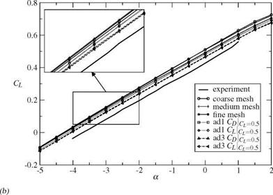
In figure 4(a) the lift is plotted as function of the angle of attack a. The results on the coarse, medium and fine mesh are denoted by о, + and *. On the coarse and medium mesh the results are similar. On the fine mesh the slope is lower than on the coarser meshes. The computed lift on the adapted meshes ad1 for lift and drag are nearly identical within the line thickness. In comparison to the fine mesh the lift is shifted by SCl « 1LC. The computed lift on the meshes ad3 show the same behaviour. Only the shift to the fine mesh is SCl « 2LC.

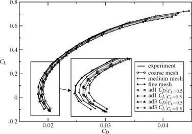
The lift as function of the drag is plotted in figure 4(b). On the refined mesh series the drag reduces by the mesh refinement. The strongest variation of the lift as function of the drag is observable in the region of minimal drag where the curve of the fine mesh is shifted to the left by SCd ~ 10DC in comparison to the drag computed on the coarse mesh. For large angles of attack the reduced drag is nearly completely compensated by the reduced values of the lift so that the curves of the refinement series are close together. For the adapted meshes the shift at the minimal drag is only 8Cd « 3 – 5DC with respect to the results on the coarse mesh. In contrast to the refined meshes the deviation for large angles of attack are getting higher by the number of points.

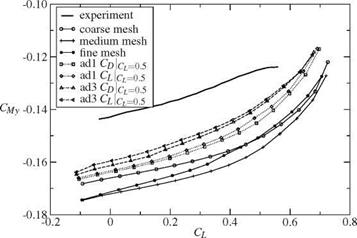
In figure 5 the pitching moment is plotted as function of the lift. The results for the refined mesh series are ambiguous and no trend is observable. The pitching moment on the adapted meshes ad1 and ad3 increases by each refinement.

DLR-F6

DLR-F6

Fig. 4 (a) Lift Cl as function of the angle of attack a and (b) polar of Cl as function of Cd for the DLR-F6 model. o, + and * denotes the results on the coarse, medium and fine mesh. □ and 0 marks the results on the first adapted mesh at Cl = 0.5 with respect to the lift and drag, respectively. Д and < denotes the results computed on the meshes of the third adaptation step of figure 3. The solid line denotes the experimental results taken from [7].

DLR-F6

DLR-F6

Fig. 5 Pitching moment Сму as function of the lift Cl for the DLR-F6 model. The labels are identical to the labels of figure 4.

The measurements of [7] are plotted in the figures 4 and 5 as a solid line. Like in the convergence study by trend the lift (angle of attack) and pitching moment of the adapted meshes fits more to the experimental results than the coefficients computed on the refined meshes. The measured lift as function of the drag fits more to the refined meshes.

Results

2.3 Adaptation by an Adjoint Error Estimate

The adjoint error estimate as sensor for adaptation is tested on two configurations. The first configuration is a clean wing/body configuration of the DLR-F6 geometry
[8, 12]. The second configuration is the high-lift wing/body configuration TC 217 with deployed flaps and slats. For both configurations the numerical results are com­pared to wind tunnel measurements.

Methods

For this study two different methods were used. The first approach solves an ad­joint problem to get an error estimate of a functional. This error estimate is used as sensor for adaptation. The second method is based on the local modification of the unstructured part of the mesh to increase the quality of the mesh. All computations were performed with the TAU solver from the DLR (Deutsches Zentrum fur Luft – und Raumfahrt).

2.1 Adjoint Error Estimation Method

The adjoint error estimation method uses a solution of an adjoint problem as sensor for an adaptation. The sensor is goal-oriented which means that for a specific goal function (e. g. CL, Cd or CMy) the sensitivity on the error of this goal-function is locally computed. Based on this error estimate the mesh is refined to improve the results with respect to the specified goal function.

The original sensor of [13] is based on an estimate for the goal function I on a globally refined mesh

Ih(UH – Ih(Uh) « {VH)TR{UH) (1)

by the adjoint у times the residuum R of the flow U, where the subscript h means results on the isotropically refined mesh, the superscript H denotes an extrapolation from the coarse to the fine mesh. So on the right hand side of (1) the adjoint у is computed on the original mesh and extrapolated to the fine mesh. The flow quantity

U is extrapolated to the fine mesh. After that the residuum is calculated on the fine mesh from this extrapolated vector.

To avoid the extrapolotion and the calculation of the residuum on the fine mesh a new sensor was developed by [2]. The idea of [2] is to assume that the major part of the discretization error comes from the dissipation error. The error estimate is then given by

<2>

The corrected value of the goal function is

+ JL). <3)

Подпись: Si,j Подпись: T Ytj Methods Подпись: ,(4) dRK Подпись: (4)

The related sensor for the adaptation is the absolute value of the local product

2.2 Mesh Manipulation

Methods Подпись: (5)

For optimizing a mesh, a quality measure for its elements has to be defined. Here the used quality measure based on the so-called mean ratio

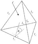
where Ai is the area, Vi the volume and lij the edge lengths of the element i (see figure 1a). Basically the measure is a ratio between the volume (3D) or area (2D) and the edge lengths.

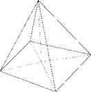
For three-dimensional cases this quality measure was extended to pyramids by splitting the pyramid into four tetrahedra by introducing a mid point on the basis of the pyramid (see figure 1b).

The implementation of the mean measure allows to use local anisotropic metrics. The modified metric can be helpful if more information about the flow e. g. a pre­liminary solution is available. In this case the orientation of the elements to the local flow is considered. Due to this new metric the edge lengths, area and volume are measured in the space of the new metric M. The size functions in the new metric are then given by

Methods
Methods

Fig. 1 (a) Nomenclature of variables on a tetrahedral element i. (b) Splitting of a pyramid into four tetrahedrons.

I’if = J(x/ – Xj)T • JC • (x/ – Xj),

(6)

А/ = yjdet {Ж

(for 2D meshes),

(7)

V-g =

(for 3D meshes).

(8)

For this study the metric was derived from the Hessian of the local Mach number

Malocal

^=^4—Ma/oca/. (9)

OXiOXj

To get a positive definite metric the Hessian was decomposed to its eigenvalues.

(h 0 0

H = R • 0 Я2 0 • RT. (10)

0 0 X3)

The new local metric is then defined by the absolute values of the eigenvalues

(ІЯ11 0 0

M = R • 0 ІЯ21 0 • RT (11)

V 0 0 ІА3)

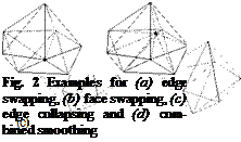
To improve the quality of a three-dimensional mesh, four different methods are implemented to modify the unstructured:

• edge swapping for up to 8 surrounding tetrahedrons [6, 10]

• face swapping [face to edge swap in 10]

• edge collapsing [9]

• combined smoothing [11, 1,4] with an optimizer for not continuously differen­tiable goal functions [5, 6, 3]

Methods Подпись: (b)
Methods
Methods
Подпись: (d)

Each method modifies the mesh locally and acts on tetrahedrons. The combined smoothing and the edge collapsing were extended to allow modifications on points connected with pyramids. An example for each method is sketched in figure 2(a)- (d). For two-dimensional grids only edge swapping and the movement of nodes are implemented.

For pointwise optimization due to movement of a node, a goal function has to be defined which combines the quality of surrounding elements Si of a node i. Here the minimal quality

g (Si)= min q} (12)

jeSi

was used as goal function for the optimizer.

A modification of the grid is tried if the geometrical constraints allow a modi­fication. Additionally the following demands have to be always fulfilled to accept a modification step:

• the minimal quality is larger than zero (to avoid inverted elements)

• the minimal quality is larger than the global minimal quality

• the goal function has to be improved (in the case of node movement)

• improve the mean quality (and therefore the global quality of the mesh)