Category A PRACTICAL. APPROACH TO. ROBUSTNESS. ANALYSIS

MARGIN

In the context of a robust stability problem, l/fi(M(jw)) represents the size of the smallest parametric uncertainty S, which brings one closed loop pole on the imaginary axis at ±ju. The robust stability margin kmax is obtained by computing the s. s.v. along the imaginary axis:

The principle is thus to detect the crossing of one of the closed loop poles through the imaginary axis. ктах corresponds to the size of the smallest parametric uncertainty 8, which brings one closed loop pole on the imaginary axis.

Remark: several reasons exist for handling the, v..v. к n(M(ju)) rather than its inverse the multiloop stability margin (m. s.m.).

As a first point, the s. s.v. can not take an infinite value, since

the nominal closed loop is asymptotically stable, whereas the m. s.m. may be infinite (if no structured model perturbation exists, which destabil­izes the closed loop). On the other hand, the s. s.v. can be considered as an extension of classical algebraic notions, namely the spectral radius and the maximal singular value of a matrix (i. e. its spectral norm – see below).

2.2 THE GENERAL CASE

The problem of extending the approach of subsection 2.1 to the case of neglected dynamics seems a priori more complex, since Д is now a dynamic transfer matrix instead of a simple gain matrix. Nevertheless, assume that a complex matrix Д0 was found, which satisfies det(I – M(ju>)A°) = 0 at frequency u>. It suffices then to find a transfer matrix A(s) with A(ju}) = Д0. When applying A(s) to the interconnection structure, a closed loop pole is obtained on the imaginary axis at ±juj.

The unit hypercube D is introduced as:

D = {J = [ft… <У I Si Є R and |<5*| < 1} (1.20)

Remember that the real model perturbation Д — — a— (—— I— ( . For the

sake of simplicity, we note with some abuse of notation Д Є D: this should be understood as 8 Є D.

Assume that the nominal closed loop is asymptotically stable, which is

equivalent to the assumption of an asymptotically stable transfer matrix M(s) (i. e. all eigenvalues of the state-matrix A are strictly inside the left half plane). The problem can then be formulated, either as a robustness test ("Is the closed loop of Figure 1.1 stable for all parametric uncer­tainties Si inside the unit hypercube D?"), or as the computation of a robustness measure ("What is the maximal value kmax of к for which the closed loop of Figure 1.1 is stable for all parametric uncertainties Si inside the hypercube kD?").

This last problem reduces to look for the smallest value of k, for which the closed loop becomes marginally stable (i. e. one or more poles on the imaginary axis and all other poles strictly inside the left half plane) for a parametric uncertainty inside kD. Assume indeed that S Є kD and let k increase from the zero value: since the nominal closed loop is asymp­totically stable, the closed loop becomes marginally stable for a value of S inside kD before being unstable (because of the continuity of the roots of the polynomial Pcl(s, S) as a function of the vector S of uncertain parameters).

On the other hand, equation (1.19) emphasizes the link between the singularity of the matrix I — M{juif)A and the presence of a closed loop pole on the imaginary axis at ±jw0.

As a consequence of the above discussion, the s. s.v. is introduced as follows. The complex matrix M in the following definition may be un­derstood as the value of the transfer matrix M(s) at s = juj.

DEFINITION 2..1 The s. s.v. n(M)associated to a complex matrix M and to a real model perturbation A, is defined as:

1

/x(M)

p(M) =0 if no A satisfies det(I – MA) = 0.

The idea is thus to find the minimal size model perturbation Д (or equi­valently S), which renders singular the matrix I — MA: the. v..v. v. p(M) is defined as the inverse of the size of this model perturbation.

We come back to the problem of subsection 1.4, namely the stability of the interconnection structure M(s) — A when A = diag(5ilqi) only contains real parametric uncertainties 8,. The problem reduces to the computation of the s. s.v. g(M(s)) along the imaginary axis, i. e. for s = jw with u> Є [0, оо].

2.1.1 A PRELIMINARY RESULT

For the sake of simplicity, M(s) is assumed to be a strictly proper transfer matrix. Let (A, B, C, 0) a state-space model ofM(s). Noting that Д may be considered as a feedback constant matrix, the state-space matrix of the closed loop M(s) — A is A + ВАС, and its characteristic polynomial is:

where 8 is the vector of parametric uncertainties associated to A — diag(8ilqi). With the classical properties det(XY) = det(YX) and det(I – XY) = det(I – YX), it is straightforward to rewrite the above equation as:

Pcl{s, 8) = det(sl – A)det(I – C(sl – A^BA) (1.18)

Since M(s) = C(sl – A)~lB and Pol{s) = det(sl – A) represents the open loop characteristic polynomial (i. e. the one associated to A — 0 and thus to the nominal closed loop M(s)), the following result is obtained:

The above equation is the specialization to the case of the interconnection structure M( s) — Д of a well known result, which is the basis of the multivariable Nyquist theorem.

The aim is to introduce in a rather qualitative way the s. s.v. as a tool for the study of the stability of a closed loop in the presence of a structured model perturbation. One focuses in this section on the stability property inside the left half plane. Other regions of the complex plane will be considered in the following section. For the sake of clarity, the first subsection presents the special case of a closed loop subject to parametric uncertainties. The general case of parametric uncertainties and neglected dynamics is treated in the second subsection. The third subsection is devoted to a technical, but practically important issue, namely the choice of the weights on the model uncertainties.

We now consider the general case of a closed loop, which is simul­taneously subject to parametric uncertainties and neglected dynamics.

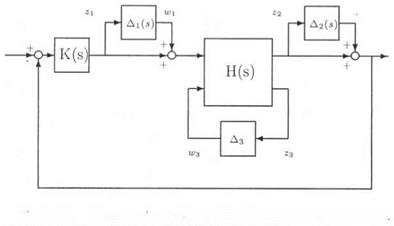
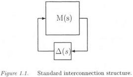
The issue is first to realize the parametrically uncertain plant model as an LFT Fi(H(s), Д3) (see subsection 1.4). The control law is then con­nected with the plant and the neglected dynamics are finally added at various locations of the closed loop. The standard interconnection struc­ture M{s) — A(s) is obtained, by noting that M(s) is the transfer matrix seen by the structured model perturbation A(s).

II’2

Figure 1.7. Computation of the standard interconnection structure

The example of Figure 1.7 combines the examples of figures 1.6 and 1.4. The parametric uncertainties are gathered in Д3 = diag(SiIqi). Д(з) has the following structure:

A(s) = diag(Ai(s),A2(s),S1Iqi,… ,SrIqr) (1.16)

whereas M(s) is the transfer matrix between (w,W2,w^) and outputs (zi, z2, z3).

• Assume as an example that the parametric uncertainties <5* enter in an affine way the state-space equations of the plant’:

x = (Ao + ^ Аі8і)х + (Bo + Bi5i)u

І І

У = (0) + £едя + (А> + £ВДг* (1.13)

І І

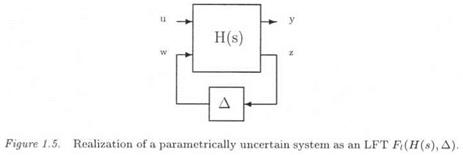
Si Є [—1,1] represents the normalized variation of the ith uncertain para­meter. Using Morton’s method (Morton and McAfoos, 1985; Morton, 1985) (see chapter 3), the uncertain plant can be transformed into an LFT у = Fi(H(s),A)u, where и and у are the physical inputs and out­puts of the plant (see equation (1.13) and Figure 1.5). Ais a diagonal matrix of the form:

The scalar Si is consequently repeated q, times, where qi is the rank of the augmented matrix Pf.

(1.15)

The idea is thus to add fictitious inputs and outputs го and z, so as to introduce then the uncertainties as an internal feedback w = Az (see Figure 1.5).

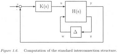
the LFT model of the uncertain plant. It suffices to connect the plant inputs and outputs u and y (see Figure 1.5) with the inputs and outputs of a controller K(s) (see Figure 1.6) to obtain the standard interconnection structure of Figure 1.1. M(s) corresponds in Figure 1.6 to the transfer matrix, which is seen by the model perturbation A, i. e. to the transfer between ги and z. Note finally that Д is no more a dynamic transfer matrix, unlike in the previous subsections. It is just a matrix gain containing real parametric uncertainties.

• Two neglected dynamics Ai(s) and A2(s) are now introduced at the plant inputs and outputs. For the sake of simplicity, associated weighting functions Wi(s) are not accounted for. These neglected dynamics may especially enable to handle simultaneously uncertainties in the actuators and sensors dynamics.

The aim is here again to transform the uncertain closed loop of Fig­ure 1.4 into the standard interconnection structure M(s) — A(s). As in the previous subsection, M(s) is the transfer matrix between the inputs (wi, w2) and outputs (z, Z2), whereas the structured model perturbation A(s) is:

In the previous subsection, A(s) was an unstructured model perturb­ation, since it corresponded to any transfer matrix satisfying the Hoo inequality (1.3). In the above equation, both Ai(s) and A2(s) are as­sumed to satisfy the Hoo inequality (1.3). There’s however an additional structural information in equation (1.9).

Remark: an unstructured model perturbation A(s) becomes at s = joj a complex matrix A(ju>) without specific structure, which simply satis­fies <( Д (juj) ) < 1 . Д « ) is said to be a full complex block. [3]

At frequency w, this unit ball becomes:

BA(jw) = {ACM = diag(Ai(ju),…, Am(jcu)) | a(A(ju)) < 1K1.12)

Because of the block diagonal structure of A, the inequalities )| A.(s) ||co < 1 andCT(A(ju;)) < 1 reduce to ||Aj(s)||oo < 1 and a(Aj(jw)) < 1 for each block of neglected dynamics.

• As in the previous subsection, the aim is to compute the maximal amount of neglected dynamics, for which the closed loop remains stable. Assuming that the nominal closed loop is asymptotically stable, the ro­bustness margin kmax is the maximal value of k, for which the closed loop remains stable in the presence of neglected dynamics Aj(s) satisfy­ing ||Aj(s)||oo < A; for j =

It is still possible to apply the small gain theorem to the above prob­lem. The result is nevertheless conservative, i. e. only a lower bound of the robustness margin kmax is obtained. Indeed, when applying the small gain theorem to the interconnection structure M(s) – A (s), the block diagonal structure of the model perturbation A(s) is not taken into ac­count, i. e. A (s) is considered as a full block of neglected dynamics.

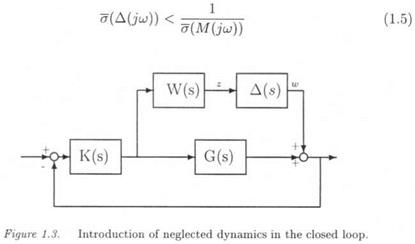
• A single block of neglected dynamics A(s) is introduced in the closed loop. Consider the example of Figure 1.3: the plant model G(s), the controller K(s) and the weighting function W(s) are known transfer matrices, while the normalized neglected dynamics A(s) correspond to an uncertain transfer matrix, which is just known to satisfy the inequality:

By definition of the Hoo norm, this relation becomes at frequency ш:

°{A(juj)) < 1 (1.4)

As a first point, the model uncertainty Д(з) is said to be additive in the context of Figure 1.3, since the true plant is modeled as (?(s)+A(s)W(s). This additive representation of the model uncertainties is especially used in the context of flexible structures, to represent an uncertainty in the bending modes dynamics. As a second point, the true uncertainty in the plant dynamics is A(s)VF(s), so that the weighting function W(s) is used to introduce our knowledge of this uncertainty in the plant dynamics (see below). [2]

• Assume that the nominal closed loop (i. e. the one corresponding to A(s) = 0) is asymptotically stable. The issue is to determine the max­imal amount of neglected dynamics, for which the closed loop remains stable. A simple solution is provided by the small gain theorem, which gives a necessary and sufficient condition of stability of the closed loop at frequency w:

As expected, if the normalized neglected dynamics A(s) satisfy equa­tion (1.4), the model uncertainty which is induced by the

reduction of the plant model, satisfies inequality (1.6).

Consider an LTI closed loop subject to parametric uncertainties and neglected dynamics. Simple examples illustrate in the following subsec­tions that it is most generally possible to transform a specific uncertain closed loop into the standard interconnection structure M(s) – A(s) of Figure 1.1: the transfer matrix M(s) contains the dynamics of the nom­inal closed loop (i. e. the closed loop without any model uncertainty) and the way the various model perturbations enter the closed loop. On the other hand, all model perturbations are gathered in the uncertain trans­fer matrix A(S). As a preliminary, the notion of LFT, which plays a key role in the Ц framework (and more generally in robust control and robustness analysis), is defined.

1.1 LFTS

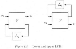
Lower and upper LFTs are defined in this subsection in a generic way. Let P, Ді, Д2 denote either transfer matrices or complex matrices: in Figure 1.2, the lower LFT F)(P, Д2) is the transfer between w and z, while the upper LFT FU(P, Ai) is the transfer between u;2 and г2. Partitioning P compatibly with the Aj’sas:

the LFTs Fi{P, Д2) and FU{P, Ai) can be written as:

Fl(P, Д2) = Pn + P2&2(I – P22&2)~XP2

Fu(P, Al) = P22+P2lbl(I-Pnbl)~lPl2 (1.2)

The chapter is organized as follows. In the first section, simple ex­amples illustrate how to transform a specific control problem into the standard interconnection structure. This qualitative presentation will be completed by a technical presentation of the associated methods in chapter 3. These techniques will be moreover applied to the aeronautical examples in chapter 4.

The s. s.v. is then introduced in a qualitative way in the second section. More precisely, we first focus on the problem of robust stability inside the left half plane. The s. s.v. provides a solution to this problem, first in the context of parametric uncertainties, and then in the general con­text of mixed uncertainties (i. e. parametric uncertainties and neglected dynamics). The third section considers robust performance problems, and shows that the s. s.v. provides a general framework for analyzing the robustness properties of a closed loop subject to model uncertainties.

The Ц framework is finally introduced in a formal way in the last sec­tion. The (skewed) s. s.v. is first defined. The Main Loop Theorem, which plays a key role in the ц approach, is then introduced, before being inter­preted in a qualitative way in the specific context of robust performance problems. Some difficulties of the ц approach are finally briefly indic­ated, and especially the need to compute bounds of the s. s.v. instead of the exact value. These difficulties will be further studied in the next chapters.