Category A PRACTICAL. APPROACH TO. ROBUSTNESS. ANALYSIS

• The difficulty of the method of subsection 1.3 is that uncertain scalars Xi are to be handled, which vary between —oo and Too. If methods ex­ist for deciding whether v0S{M{ju>)) is less than a given strictly positive value at a fixed frequency w (see e. g. the previous subsection), it is not so obvious to decide whether v0S(M{juj)) is zero, especially when bounds of Ms ( M j w ) ) are computed instead of the exact value.

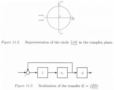
On the other hand, it would be more convenient to represent the fre­quency response e-^T> with a real non repeated scalar. As a first reason, the computational methods of the previous subsection are difficult to ex­tend to the case of real repeated scalars. As a second and more import­ant reason, the gap between the bounds tends to increase with repeated scalars. Nevertheless, this requirement imposes to split the circle corres­ponding to e~^T into two half circles (see Figure 11.2): the bottom half circle (between 1 and -1) and the top half circle (between -1 and 1).

• In this context, the uncertain scalar Xi is rewritten as:

so that aj Є [0, 1] corresponds to Xi X [0, X oo)? i. e. to the bottom half circle. As a consequence:

with:

As in subsection 1.3, the model perturbation Д2 = diag{5{,…, 6CN) can be rewritten as an LFT F^W., Д2), where:

Д2 = diag(ai,… ,aN) (11.17)

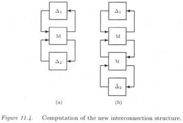
Here again, the initial interconnection structure M – Д of Figure 11.4.a is transformed into the new equivalent interconnection structure M — Д of Figure 11.4.b, where M = M and Д = diag(A, Д2).

An upper bound of u°£{M{ju))) is now to be computed. If this upper bound is strictly greater than 1, a lower bound of the robust delay mar­gin can be deduced. An upper bound of this margin can also be obtained with a lower bound of u^(M(ju)).

• If the upper bound ofv^(M(jco)) is less than 1 at the previous step, no destabilizing value of the delays can be found on the bottom half circle. The delay frequency response is thus rewritten as:

1 , p _ Іхі ~ 1 = -1 + (1 + j)aj

1 jXi + l 1 + (j – l)«f —2(1 — qj)

1 – «і 4- jcti

with:

The top half circle (between -1 and 1) is obtained when сц є [0, 1]. As above, a new interconnection structure M — A is computed, in which the model perturbation Д contains the original mixed model perturbation Ді and the real non repeated scalars aj’s.

An upper bound of u^(M(ju)) is calculated. If it is less than 1, an infinite robust delay margin is obtained. Otherwise, a lower bound of this margin is deduced. In this case, an upper bound of the margin can also be obtained with a lower bound of

Remark: the interest of the above method is that it is geometrically very simple. See nevertheless (Scorletti, 1997) for a more complex, but potentially richer method.

2.1 COMPUTATION OF uos BOUNDS

The methods of subsections 1.1 and 1.2 (chapter 5) are briefly extended to the computation of a bound of where M is a complex matrix

and Д = Дag( Д і, Д2 ) contains only real non repeated scalars. The idea is simply to note that vertices (resp. two-dimensional faces) are handled in the method of subsection 1.1 (resp. 1.2). Let 6 a vector of parametric uncertainties. Two cases are to be considered:

1. 6 is to be expanded inside its one-sided unit ball BAos.

2. <5 is to be maintained inside its unit ball (i. e. the unit hypercube D).

In the context of the method of subsection 1.1 (chapter 5), remember that all scalar components 5- of a vertex Sl take an extreme value. In the first case above, this means that S is chosen as = 0 or S — k. In the second case, Jj ± 1.

In the context of the method of subsection 1.2 (chapter 5), 8 belongs to a two dimensional face of the hypercube if all its components take an extreme value, except two ones. The extreme values are chosen in the same way as above. The two other components 5i and Sj are obtained as in subsection 1.2 (chapter 5). In the first case, 8 is an acceptable solution if Si and Sj belong to the interval [0, k] . In the second case, S is acceptable when Si and Sj are inside [-1, 1].

Remark: both methods above are exponential time, and they are applic­able to problems with a few parametric uncertainties and delays, which is the case of the missile example of section 4.. See (Ferreres et al., 1996b) for the computation of a polynomial time upper bound of

The aim of this subsection is to present the principle of the method in a qualitative way: see the following section for a detailed algorithm.

•LetM(s)- A(s) the standard interconnection structure, with Д(в) = diag(Ai(s), A2(s)). Remember Ai(s) is a mixed model perturbation gathering all classical model uncertainties, whereas Дг(а) gathers all un­certain time delays (see equation (11.4)).

Assuming that the nominal closed loop (i. e. the closed loop without time delays and model uncertainties) is asymptotically stable and with reference to the Nyquist stability criterion (Ferreres and Scorletti, 1998), the key point is to note that the analysis of the robust stability property of the closed loop reduces to the problem of detecting at each frequency и the singularity of the matrix I — M(juj)A(ju), i. e.:

det(I – M{jw)diag{A(ju),e~^UTl – 1,… ,e~j“TN – 1) = 0 (11.7)

The frequency u> is fixed in the following, and the w dependence is drop out, so that M and Д = diag(Aі, Д2) mean the values of M(s) and Д($) = diag(Ai(s), Д2(я)) at s = ju>.

constraint (e. g. |<5гс| < 1). This explains why conservative results are obtained with this method, even if the exact value of /л is computed.

In order to fully take into account this information and with reference to the bilinear transformation, the idea is simply to rewrite the complex

scalars S£ ’ s as:

where j2 — — 1 and the real scalar хг belongs to the interval [—oo, +oo] (see Figure 11.2). The magnitude of 1 + Sf is now constrained to be 1, and a real scalar X{ is to be handled. Sf is thus (see also Figure 11.3 for an LFT realization):

• We come back to the initial interconnection structure M – Д, with Д = diag(Aі, Д2). With reference to equations (11.8) and (11.10), each complex scalar S is rewritten as an LFT Fi(H, Xi), with:

In the same way, the model perturbation Д s is rewritten as 2),

where:

Д2 = diag{xi,…,xN)

As a consequence, the initial interconnection structure Д – Д of Fig­ure 11.4.a can be transformed into the new equivalent interconnection structure M—A of Figure 11.4.b, where M = M[12]H and A = diag(A 1, A2) (see subsection 3.1 of chapter 3 for the definition of the star product M-kH). The interconnection of LFTs is indeed an LFT.

Remark: consider the problem of checking whether a template on a closed loop transfer function remains satisfied despite classical model uncertainties (parametric uncertainties and neglected dynamics). Fol­lowing chapter 1 (section 4.4), this classical robust performance prob­lem can be converted into an augmented stability problem, in which a full complex block is added to the structured model perturbation. As a consequence, the method described in this section can be extended to the problem of checking whether a template on a closed loop trans­fer function remains satisfied despite parametric uncertainties, neglected dynamics and delays.

For the sake of clarity, the method is introduced with the following gen­eric example. Let G(s, 6) the uncertain plant model, i. e. aMIMO transfer matrix which depends on a vector 8 of parametric uncertainties. Follow­ing chapter 3, G(s,8) can be transformed into an LFT Fi(P(s), Ai), where:

is a model perturbation with real possibly repeated scalars <5*.

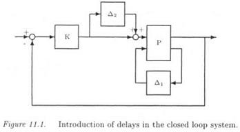
Controller K(s) is connected with G(s,8) and a model perturbation Д2(з) is added at the plant inputs (see Figure 11.1). Д2(з) represents the uncertain time delays:

Д2(в) = diag(e~ns — 1,…, e~TNS — 1) (11.4)

This uncertain closed loop is finally transformed into the standard in­terconnection structure M(s) – A(s). M(s) is simply the transfer matrix seen by the model perturbation A(s) = diag(Ai, ДгЫ) in the closed loop of Figure 11.1.

Remark: other examples could be considered, since other sources of parametric uncertainty or neglected dynamics could be introduced at various points of the closed loop (see chapter 1). Time delays could be moreover introduced at the plant outputs, in order to take into account delays in the sensors. The key issue is to obtain the standard intercon­nection structure M(s) – A(s),with A(s) = diag(Ai(s), A2(s)). Ai(s) is a mixed model perturbation gathering all classical model uncertainties (parametric uncertainties and neglected dynamics), whereas the model perturbation ДгЫ contains all uncertain time delays.

The robust delay margin is now defined in the specific context of the example. Assume that each parametric uncertainty Si is normalized, so that the vector S = (й)іє[і, м] belongs to the unit hypercube:

D = {6 – 1 < Si < 1 Vi Є (11.5)

A specific value of 6 is applied to the closed loop of Figure 11.1. Let Дт(<5) the MIMO delay margin associated to this closed loop: this means that the robust stability of the closed loop is guaranteed for all values of time delays Tj inside the interval [0, Дт(£)]. The robust MIMO delay margin At* is then defined as the minimal value of Дт(<5) over the unit hypercube[11]:

At* = min Дт(5) (11,6)

The problem of analyzing the robustness properties of a closed loop in the presence of classical model uncertainties (parametric uncertain­ties and neglected dynamics) and uncertain time delays presents a great practical interest. Indeed, when embedding control laws on a real-time computer, time delays are to be accounted for at the plant inputs (be­cause of the time needed for computing the value of the plant input signal as a function of the plant output signal) and outputs (because of the sensors which measure the plant output signal).

The aim of this chapter is to provide an algorithm for computing a robust delay margin: see (Ferreres and Scorletti, 1998) for a complete theoretical justification. The method is presented in a qualitative way in the first section. The second section details the computational al­gorithm. An alternative small gain approach is presented in the third section. Both methods are compared on the missile problem in the fourth section: time delays are added at the input and outputs and uncertainties in the stability derivatives are considered.

1. INTRODUCTION TO THE PROBLEM

A frequency dependent test is introduced, whose resolution at each frequency essentially reduces to a ц problem with a specific structure (namely a one-sided skewed /і problem). If the exact value of p could be computed, the exact value of the robust delay margin could be obtained.

1.1 A ONE-SIDED SKEWED ц PROBLEM

As an extension of the classical s. s. v. v, the one-sided skewed s. s.v. v^(M) of a complex matrix M is defined (Ferreres et al., 1996b). In the stand-

ard interconnection structure M — Д, the uncertainty Д is split as Д = diag{Aі, Дг)- Ді is a mixed perturbation, while Д2 contains real (pos­sibly repeated) scalars £[:

Д2 = diag(8ri Iki) (11.1)

Let the one-sided unit ball BA™:

BA°2s = {Д2 = diag{8llki) / 8 Є [0,1], і = 1,… ,mr} (11.2) DEFINITION 1..1

v™(M) = l/min(k / ЭД = diag(A, /гД2) with Д2 Є BA™,

A Є BA and det{I — МД) = 0)

= 0 if no (/с, Ді, Д2) exists

The issue is to check the validity of the 13th order controller on the full 46th order plant. Uncertainties are introduced in the natural fre­quencies of the 20 bending modes contained in the identified telescope model: see chapter 2 (section 3.) for the presentation of the mock-up and chapter 4 (section 2.2) for the computation of the LFT model. A model perturbation with 20 non repeated real scalars is to be handled.

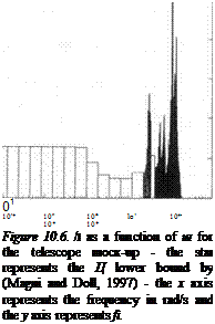
The basic algorithm of subsection 5.1 is first applied. Results are shown on Figure 10.6, which displays the fj, upper bound as a function of frequency. Note first the very fine peaks on the /і plot. An upper bound of the maximal s. s.v. over the frequency, interval [0, 1600 rad/s] is obtained as 46.80, between 1101.75 rad/s and 1103.95 rad/s. The H<i controller can thus tolerate an uncertainty of only ±2 % (и 1/46.8) in the frequencies of the bending modes. The star on Figure 10.6 corres­ponds to the Ц lower bound by (Magni and Doll, 1997), namely 44.94 at

1103.4 rad/s. The gap between the bounds is less than 4%, the result is nearly non conservative.

The associated computations were achieved in 14776s (about 4 hours) on an efficient Sun SPARCstation. If the aim is just to compute an upper bound of the maximal s. s.v., the improved algorithm of subsection 5.2 can be applied. All frequency intervals are eliminated, except the one between 1097.34 rad/s and 1114.98 rad/s. The basic algorithm is then applied to this single interval, and the same value is obtained for the upper bound of the maximal s. s.v., namely 46.80 between 1101.75 rad/s and 1103.95 rad/s. The associated computations were achieved in 3210 s (less than an hour).

50 – 45 – 40 – 35 – 30 – 25 – 20 – 15 – 10 –

5 –

For both algorithms, the computational requirement is thus not neg­ligible in the case of this example. Nevertheless, the computed value of the robustness margin is reliable, in the sense that it can be guaranteed that a critical peak on the ц plot was not missed. The result is moreover
nearly non conservative, and the telescope problem is quite challenging: the more flexible the example, the heavier the computational burden. In the case of very lightly damped flexible modes, the frequency intervals have to be chosen very small to detect very narrow and high peaks on the /г plot. In practice, the computational burden simultaneously de­pends on the structure of the model perturbation (this burden increases with the complexity of this structure – 20 real scalars in the case of this example), on the values of the damping ratios of the bending modes (roughly between 0.2 % and 2 % in the case of this example) and on the number of these bending modes (20 modes in the case of this example).

Let ] і і+і ] the critical frequency interval, which correspond to the maximal value of the /supper bound (namely [9.93 rad/s, 10.00 rad/s]). When choosing as a frequency gridding a few points between і and Wj+i, it is interesting to point out that the same result is obtained with all three methods. The lower bound is 1.966 and the critical frequency is 9.95 rad/s.

CONCLUSION

Two different cases are to be considered: if the method of subsection

5.1 has been already applied or if our physical knowledge of the problem enables to predict the frequency domains corresponding to the peaks on the fi plot, methods (1) or (2) are the most suitable ones, since they give good results while being very simple to implement. Otherwise, if no guess of the critical frequency domains is available, method (3) is especially attractive, since it seemingly enables to detect the peaks on the і plot, even when using a rough frequency gridding (at least in the case of the example). Moreover, remember that the improved algorithm of subsection 5.2 assumes that a t1 lower bound of good quality is a priori available. When applying method (3) on a rough frequency gridding, such a lower bound may be obtained, and the associated computational burden remains reasonable.

This subsection compares the results obtained with the three methods proposed in chapter 5 (section 3.). A rough frequency gridding is first considered. The three methods are then evaluated around the critical frequency.

6.1.1 USE OF A ROUGH FREQUENCY GRIDDING

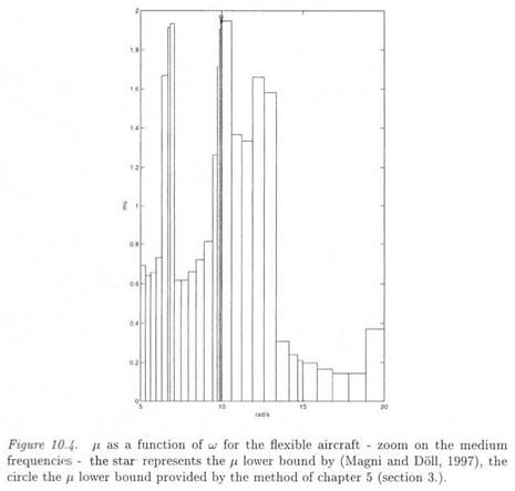
The frequency gridding is chosen as a set of 30 points logarithmically spaced between 0.01 rad/s and 100 rad/s. The results are presented in the above table. It is especially worth emphasizing that methods (1) and (2) only detect a single peak, while the third method, which is based on Linear Programming, detects the two most critical peaks (these ones also appear in Figure 10.4).

The improved algorithm of subsection 5.2 is applied. Most of the frequency intervals, which correspond to the 50 points of the initial fre­quency gridding, were eliminated, and the basic algorithm of subsec­tion 5.1 is applied only to 8 intervals. The same result is obtained for Umax – The computations were done in only 474 s (about 8 minutes). This improved solution appears thus especially computationally efficient. Moreover, the result is nearly non conservative.

6.1 A PHYSICAL INTERPRETATION OF THE ti LOWER BOUND

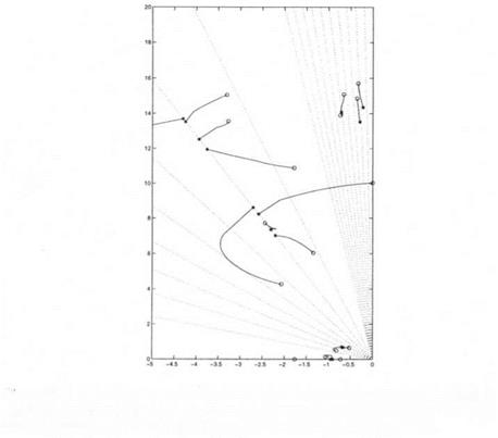
The aim of this subsection is to illustrate the usefulness of a q lower bound. Let (А, В, C, 0) a state-space representation of the transfer mat­rix M(s) in the interconnection structure M(s) – Д. A destabilizing perturbation Д* is provided with the fi lower bound. Remember that the value of this lower bound is 1.94 at 9.97 rad/s with the method by (Magni and Doll, 1997). This means that the norm of Д* is 1/1.94 and that the closed loop state matrix A + BA*Chas a pole on the imaginary axis at ± 9.97 rad/s.

This is confirmed by the root locus of Figure 10.5. This root locus
was obtained by plotting the eigenvalues of A + BaA*Cwhen a varies between 0 and 1. The star "*" represents the initial poles (associated to a = 0), while the circle "o" represents the final poles (associated to a = 1). The closed loop rigid poles at the bottom of the Figure are not especially moved by the application of the destabilizing perturbation Д*.

Root locus associated to the destabilizing model perturbation, which is

provided with the fi lower bound – the dotted lines each correspond to an isovalue of the damping ratio, namely 1 %, 2 %, … ,10 % and 10 %, 20 %, … ,100 %.

The 2 closed loop flexible modes, which are not actively controlled (see subsection 1.4 of chapter 2), are neither especially moved by the application of A*. Note that two poles are associated to each flexible mode in the figure: one for the state-feedback controller and one for the observer. These two poles do not coincide, even if they are close, because the state-feedback and observer gains were computed with two different methods.

The 4 closed loop flexible modes, which are actively controlled, are

moved indeed by the application of Д*. The closed loop flexible pole, which crosses the imaginary axis, corresponds to the state-feedback closed loop pole:

frequency (rad/s)

-2.59Є+00 + 8.23e+00i 3.00e-01 8.62e+00

-2.59e+00 – 8.23e+00i 3.00e-01 8.62e+00

and thus to the open loop flexible mode:

damping

-4.39Є-01 + 8.6ІЄ+00І 5.09Є-02

-4.39e-01 – 8.61e+00i 5.09e-02

This suggests that the robustness of the observed state-feedback control­ler could be increased by improving the robustness with respect to an uncertainty in the characteristics of this critical bending mode.

As explained in chapter 4 (section 2.), uncertainties are simultaneously introduced in the 14 stability derivatives and in the natural frequencies of the 6 bending modes, whose natural frequencies are 7.35, 8.62, 12.5, 13.5, 14.1 and 14.3 rad/s. The weights in the stability derivatives are chosen as 10 %, while the weights in the frequencies are chosen as 20 %. The model perturbation contains 20 real non repeated scalars.

The basic algorithm of subsection 5.1 is first applied. 50 points were chosen for the initial gridding, namely 25 points between 0.01 and 100 rad/s and 25 points between 5 and 20 rad/s. The results are presented in figures 10.3 and 10.4. The value of the upper bound of Umax is 1.97 (between 9.93 and 10.00 rad/s): the flight control system can thus toler­ate an uncertainty of 5.1 % (~ 10/1.97) in the stability derivatives and an uncertainty of 10.2 % (и 20/1.97) in the frequencies of the bending modes. The value of the lower bound provided by (Magni and Doll, 1997) is 1.94 at 9.97 rad/s (this lower bound is represented as a "*" in figures

10.3 and 10.4). The gap between the /і bounds is consequently less than 2 %. The computations were done in 1700 s (about half an hour) on an efficient Sun SPARCstation.

A lower bound of the maximal s. s.v. over the frequency range is com­puted with the method of section 3. of chapter 5 (see subsection 6.4 for details). The frequency gridding is simply chosen as 20 points between 9.93 and 10.00 rad/s, since the maximal value of the upper bound of цтах was found inside this interval. The value of the lower bound is 1.966 at 9.95 rad/s (this lower bound is represented as a "o" in figures 10.3 and 10.4). The result is thus even more accurate than the one provided by (Magni and Doll, 1997).