Category A PRACTICAL. APPROACH TO. ROBUSTNESS. ANALYSIS

APPLICATION TO THE FLEXIBLE AIRCRAFT

APPLICATION TO THE FLEXIBLE AIRCRAFT

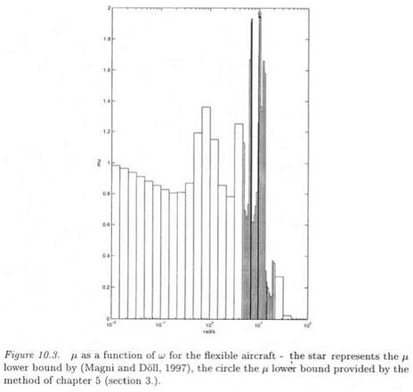
Following chapter 4 (section 2.), two methods are available for in­troducing uncertainties in the frequencies of the bending modes. Each uncertainty is represented, either by a non repeated real scalar, or by a

twice repeated real scalar. Both representations give nearly equivalent results in the following: we consequently present the results obtained with the simplest representation, i. e. the one with non repeated real scalars.

AN IMPROVEMENT

In the above algorithm, if the aim is just to compute an upper bound of Umax, it is unnecessary to apply the method of subsection 3.1 to all intervals [tup Wi+і]. Assume indeed that a lower bound 7 of цтах was a priori computed (i. e. before applying the algorithm of the previous sub­section). If the s. s.v. is proved to be less than7 on afrequency

interval [<u, tu], the critical frequency (which corresponds to the maximal s. s.v. mmax over the frequency range) does not belong to this interval. It is thus useless to apply the algorithm of the previous subsection to this interval.

Подпись: n(M{jw)) is less than m on a frequency interval [cu, ta].The issue is to find a computationally cheap method for checking whether the s. s.v.

A solution is to proceed as follows (see also (Magni et al., 1999) for an alternative method): ■ Let a frequency point tao, which may belong to the gridding

AN IMPROVEMENT

in the algorithm of the previous subsection. Find (sub)optimal values of І), G scaling matrices, which minimize the singular value:

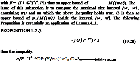
with F = (I + G2) 1^4. Remember that 7 is fixed.

Подпись:If the singular value above is found to be less than unity, apply the method of subsection inside which the s. s.v. desire to minimize the singular value in equation (10.38) should be understood as an heuristic way to maximize the size of the interval [w, її].

The issue is thus to minimize to some extent the singular value in equa­tion (10.38). In the aircraft example of the following section, the minim­ization was done as follows (see also subsection 2.4 of chapter 8):

■ Computation of a suboptimal diagonal І) scaling matrix, which min­imizes to a large extent —), with the Perron eigenvector

approach: see (Safonov, 1982). The method is computationally effi­cient and yet accurate. A routine is moreover available in the Robust Control Toolbox of Matlab.

■ Computation of an initial value of the G scaling matrix with the idea of (Young et al., 1995). Loosely speaking, the idea is simply to cancel

with G the skewed hermitian part of the blocks of —, which

correspond to the real parametric uncertainties.

■ A simple gradient method further minimizes the quantity in equation (10.38) with respect to G. Note that this quantity is not necessarily differentiable, and that the optimization problem is seemingly non convex with respect to G. It is thus important to have a good initial guess for G.

Despite its roughness, the method above gave quite good results in the example. Nevertheless, more sophisticated methods could be investig­ated, with the constraint to remain computationally cheap. Otherwise, the best solution would be to apply the basic algorithm of the previous

134 A PRACTICAL APPROACH TO ROBUSTNESS ANALYSIS subsection.

Remark: the idea of reducing the computational burden by elimin­ating frequency intervals, which can not contain the critical frequency, can be traced back at least to (Ferreres et al., 1996b). Nevertheless, this reference uses the augmented fi problem, in which the frequency is treated as an additional uncertainty. The approach proposed here is computationally much cheaper.

AN ALGORITHM THE BASIC ALGORITHM

The issue is to compute the maximal s. s.v. n(M(ju>)) over a large frequency interval [camjn, штах- Let:

Emax = max u{M{ju)) (10.37)

^€[^тгп» Mjnax]

The basic algorithm consists in the following steps:

AN ALGORITHM THE BASIC ALGORITHMis split into a set of small frequency intervals [щ, uij+i]

• The method of subsection 3.1 is applied to each interval [tup Wj+і]. The validity of the computed D, G scaling matrices on the interval is checked with the method of subsection 4.3. If the scaling matrices are indeed valid on [wj, а Ц upper bound Pi is found on this interval, and nothing

more is to be done inside [tap tuj+і]. Otherwise, the interval is split into two smaller intervals [tap (taj + u>i+i)/2] and [(w* + ші+і)/2, u>i+i],and the method of subsection 3.1 is applied to each of these two intervals. This process of branching on the frequency is repeated until а ц upper bound Pj is found on each frequency interval [tup Uj+i], whose union gives the large initial frequency interval [camjn, wmM].

• A reliable upper bound of Umax is the maximal value of the Pi’s. Either the state-space method by (Magni and Doll, 1997), or the frequency – domain method of chapter 5 (section 3.) provides a lower bound of цтах- If the gap between the bounds is not sufficiently small, it is possible to further branch on the frequency, in order to decrease the value of the upper bound of Umax-

CHECKING THE VALIDITY OF D, G SCALING MATRICES

Consider Дб? scaling matrices, which satisfy at frequency wo:

( DM {jwo)D~l

  CHECKING THE VALIDITY OF D, G SCALING MATRICES

– )G F-1/4) < 1


(10.27)


p

  CHECKING THE VALIDITY OF D, G SCALING MATRICES CHECKING THE VALIDITY OF D, G SCALING MATRICES

and:


Let then:


CHECKING THE VALIDITY OF D, G SCALING MATRICES

Let tjm the real negative eigenvalue of % of maximal magnitude. Then:

1

uj = u)q H–

Vm


CHECKING THE VALIDITY OF D, G SCALING MATRICES

(10.34)

Let then r}p the real positive eigenvalue of mi of maximal magnitude. Then:

Подпись: (10.35)_ 1

u> = loq H

Op

Proof:

CHECKING THE VALIDITY OF D, G SCALING MATRICES

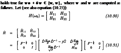
• Note as a preliminary that (see equation (10.31)):

and:

Fi(H(uo), 6ulm) = Hu + 6uHl2{Im ~ 6ljH22)-1H21 (10.36)

As a consequence:

F~1/4 1 _ f_1/4 = Ріфл6шІт) [10]

. INTRODUCTION OF THE FREQUENCY

Figwe 10.2. Introduction of frequency as a parametric uncertainty.

In order to apply the previous Lemma, an LFT model is to be derived for the dynamic system M(s), in which the frequency appears as a real parameter. The issue is more precisely to determine a complex matrix H such that, for a given strictly positive frequency uiq:

M(j(uj0 + 6u>)) = Fi(H(loq), Swim) V6u> > – loq (10.19)

Let (A, B,C, D) a state-space representation of M (s), and m the dimen­sion of matrix A. It is well known that (see Figure 10.2 with s = j(uiQ + 6ш)):

/6u>-ui0, M(j(uJo + Sui)) = F,(Mo, 7™ ) (Ю.20)

V шо + дш/

. INTRODUCTION OF THE FREQUENCY

with:

. INTRODUCTION OF THE FREQUENCY

Further note that:

with:

Подпись:T= — ( Ir? Ijp )

CUq V lm *m)

As a consequence:

. INTRODUCTION OF THE FREQUENCY

. INTRODUCTION OF THE FREQUENCY

where H(h ) is the star product of Mo and T (see subsection 3.1 of chapter 3):

. INTRODUCTION OF THE FREQUENCY

Interestingly, the LFT Fi(H(wo),SwIm) remains well-posed for Sw =


Fi(H(u0), – щіт) = D — CA~lB = M{0) (10.26)

Equation (10.19) is thus valid for all 8w > —wo.

CHECKING A POSTERIORI THE VALIDITY OF D, G SCALING MATRICES ON A FREQUENCY INTERVAL

A technical Lemma, which is the basis of this section and coincides with Lemma 2..4 of chapter 8, is presented in the first subsection. The second subsection proposes a method for introducing the frequency ш as an additional uncertainty (see section 3. of chapter 7 for alternative meth­ods). The technique for checking the validity of D, G scaling matrices on a frequency interval is finally presented in the third subsection.

3.3 A TECHNICAL RESULT

CHECKING A POSTERIORI THE VALIDITY OF D, G SCALING MATRICES ON A FREQUENCY INTERVAL

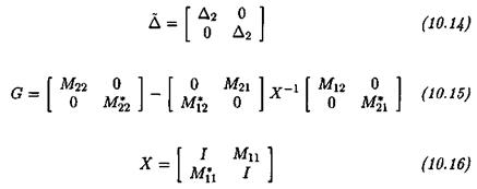
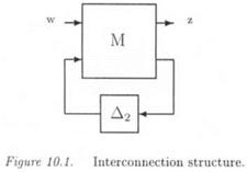
Let Fi(M, A2) the LFT transfer between w and z in Figure 10.1. Д2 is a real diagonal model perturbation, whereas the complex matrix M is partitioned as:

The transfer between w and z is thus:

Подпись:

CHECKING A POSTERIORI THE VALIDITY OF D, G SCALING MATRICES ON A FREQUENCY INTERVAL

Fi(M, Д2) = Mu + Mi2A2{I — М22Д2)_1М2і LEMMA 4..1 Let:

Assume that а(Мц) < 1 and let к < 1//^д2(М22)- Then:

a(Fi{M, Д2)) < 1 УД2 Є кВА2 (10.17)

if and only if:

CHECKING A POSTERIORI THE VALIDITY OF D, G SCALING MATRICES ON A FREQUENCY INTERVAL

det(I – AG) ф 0 УД2 Є kBA2 (10.18)

A THEORETICAL JUSTIFICATION OF THE APPROACH

A THEORETICAL JUSTIFICATION OF THE APPROACH

Let D and G some scaling matrices satisfying equation (10.6) at two frequencies u) and u>2- Let D and G the corresponding scaling matrices, computed with Lemma 2..1. D and G thus satisfy:

with F = In + G2. Assume that uj and ш2 are sufficiently close, so that a first order approximation of M(jul) is valid:

M(j((jj + (1 — A)u>2)) и XM(jbj) + (1 — )M(jw2) V А Є [0, 1]

The spectral norm a is convex, i. e. the following relation is satisfied for А Є [0, 1]:

сг(АЯ! + (1 – A)H2) < Аст(Яі) + (1 – A)a(H2) (10.10)

where Hi and Н4 are any fixed matrices. Equation (10.9) consequently implies that (V А Є [0, 1]):

A THEORETICAL JUSTIFICATION OF THE APPROACH

As a consequence, (D, G) scaling matrices, synthesized on frequencies u>і and u>2, are valid on the whole segment [wi, шг] when a first order approximation of M(jut) is valid on this frequency interval.

3.2 CONCLUSION

A first solution is to choose a sufficiently fine frequency gridding (ші)іє[і, лг]> so that the first order condition of subsection 3.2 is satisfied at all points of the frequency gridding:

+ (1 – A)wi+1)) » Ш(М) + (1 – X)M(jwi+i) VA Є [0, 1]

(D, G) scaling matrices are then computed, which simultaneously work at frequencies щ and u>j+i, in order to compute (D, G) scaling matrices, which are valid on the whole interval [w*, cuj+i].

Nevertheless, this approach will often need an unnecessarily fine fre­quency gridding, since the above equation is just a sufficient condition for guaranteeing the property that (D, G) scaling matrices, which simultan­eously work at frequencies щ and ші+i, also work on the corresponding interval. An alternative solution is to choose a looser frequency grid­ding (u>i)ie[i, jv]: (D, G) scaling matrices, which simultaneously work at frequencies and are here again computed, and the validity of these D, G scaling matrices on the frequency segment is checked only a posteriori. In this new context, a solution is to use Proposition 4..2 of the following section.

COMPUTATION OF D, G SCALING

MATRICES AT TWO FREQUENCIES

3.1 THE LMI PROBLEM

Let the complex matrices Mi = M==i ) and M2 = M(==( . Let A a structured model perturbation. The issue is to find the minimal positive value of scalar (3, for which there exist scaling matrices A A A and G Є G satisfying:

MlDM + j(GM – M*G) < (32D

М2 DM2 + j{GM2 – M%G) < /32D (10.6)

Подпись: A{D,G) = Подпись: 0 М2DM2 + j(GM2 - MiG) Подпись: (10.7)

This is a well posed generalized eigenvalue problem, which consists in finding the minimal value of /3 satisfying A(D, G) < /3213(D), with:

Подпись: M'DMi + j(GMi - MIG) 0

and:

Remark: when comparing the above LMI problem with the one asso­ciated to the mixed /j, upper bound of (Fan et al., 1991) (see equation

(10.1) ), the number of constraints is increased, but the number of op­timization parameters is the same.

2. RELATIONSHIP BETWEEN BOTH FORMULATIONS OF THE ц UPPER BOUND

The reader is referred to chapter 5 (subsection 2.3) for a presentation of both formulations of the mixed ц upper bound of (Fan et al., 1991; Young et al., 1995). The following Lemma is extracted from (Young et al., 1995). It is worth pointing out that the transformations in the Lemma below (from (D, G) to (D, G) and from (D, G) to (D, G)) do not depend on the complex matrix M.

2. RELATIONSHIP BETWEEN BOTH FORMULATIONS OF THE ц UPPER BOUND

LEMMA 2..1 Let:

with F = IN + G2. Assume that D € D and G Є Q satisfy equation

(10.1) . Let:

Подпись: (10.3)D = P

Подпись: aG = W*D-iGD~kr

2. RELATIONSHIP BETWEEN BOTH FORMULATIONS OF THE ц UPPER BOUND

where the unitary matrix U and the hermitian positive definite matrix P result from the polar decomposition:

Then D Є D and G Є G satisfy equation (10.2). Conversely, assume that D Є D and G Є G satisfy equation (10.2). Let:

Подпись:D = DF~2D G = pDGF-tD

Then D Q D and D Q Q satisfy equation (10.1).

ROBUSTNESS ANALYSIS OF FLEXIBLE STRUCTURES

1. INTRODUCTION

The previous chapters emphasized the usefulness and efficiency of the H analysis techniques. Nevertheless, as remarked in chapter 7 (section

3. ), the application of these techniques is unreliable in specific fields, such as the control of flexible structures.

Remember indeed that the principle of ц analysis is to compute the s. s.v. as a function of frequency^: the robustness margin is then

deduced as the inverse of the maximal s. s.v. over the frequency range. In practice, the s. s.v. ш)) is usually computed at each point of a frequency gridding. This technique is however unreliable in the case of narrow and high peaks on the ц plot, since it becomes possible to miss the critical frequency (i. e. the frequency for which the maximal s. s.v. is obtained may lie between two points of the gridding), and thus to overevaluate the robustness margin. This problem especially arises in the case of flexible systems (Freudenberg and Morton, 1992). As a consequence, there has been a regain of interest for robustness analysis techniques, which do not use a frequency gridding: see e. g. (Ly et al., 1994).

The solution proposed in chapter 7 (section 3.) consists in transforming a classical frequency dependent ц analysis problem into an augmented skewed n problem, in which the frequency и appears as an additional uncertainty (namely a real repeated scalar). It becomes then possible to directly compute the maximal s. s.v. over a frequency interval [u>, £3]. Two problems however arise:

■ Because of the NP hard characteristics of the fi problem, an upper bound is computed instead of the exact value of /і. In order to reduce the conservatism of this upper bound, which is calculated for the
augmented pi problem, it is more interesting to consider a set of small intervals [wj, ші+i] instead of a large frequency interval [u>, Щ.

ROBUSTNESS ANALYSIS OF FLEXIBLE STRUCTURESThe size of the augmented pi problem (which is to compute the max­imal s. s.v. pi(u) over an interval [и,, Wj+i]) can be much larger than the size of the original problem (the computation of the s. s.v. , (g ) at a fixed frequency a»). With reference to subsection 2.3 of chapter 5, remember that the problem of computing the pi upper bound of (Fan et al., 1991) reduces to an LMI problem, in which the optimization parameters are scaling matrices D and G. The computation of the optimal D, G scaling matrices for the augmented pi problem can be a computationally (very) involving task: more precisely, with reference to Lemma 3..1 of chapter 7, the model perturbation corresponding to the augmented pi problem contains the initial model uncertainties and the frequency. The associated D, G scaling matrices can thus be split into the D,G scaling matrices, corresponding to the uncertain fre­quency, and the D2 , D2 scaling matrices corresponding to the initial model uncertainties. The computational burden of the augmented pi problem is often very heavy, because the D,, G, scaling matrices contain numerous optimization parameters of the LMI problem: the uncertain frequency appears indeed as a repeated real scalar Su)Im, where m denotes the order of the state-space model of M(s) in the standard interconnection structure M(s) – Д.

An alternative solution was proposed in e. g. (Feron, 1997; Gahinet et al., 1995). The idea is to synthesize D, G scaling matrices, which simultan­eously work at two neighboring frequencies wi and u>2- Since this method does not use the augmented pi problem above, the computational burden is expected to be much lower. Moreover, this heuristic technique can be theoretically justified: it is proved indeed that when the frequencies ш and D2 are sufficiently close (in a sense which will be precisely defined in the following), the D, G scaling matrices work on the whole segment, defined by its two extremal frequencies ш and a>2.

Even when the frequencies u>i and G2 are not a priori sufficiently close, D, G scaling matrices can be synthesized, which simultaneously work at these two frequencies, and it is checked a posteriori whether the D, G scaling matrices work indeed on the whole segment. This chapter es­pecially proposes an easy and yet rigorous method, for solving this last problem of checking the validity of D, G scaling matrices on the whole segment. This method essentially relies on the alternative formulation of the mixed pt upper bound of (Fan et al., 1991), which was proposed in (Young et al., 1995).

The technique is finally applied to the flexible airplane problem (Fer-
reres and Biannic, 1998b) and to the telescope mock-up (Ferreres et al., 1998). See also (Magni et al., 1999) for an alternative technique, which is complementary to the one proposed here. The chapter is organized as follows. The relationship between both formulations of the mixed p, upper bound of (Fan et al., 1991; Young et al., 1995) is clarified in the second section. The basis of the method is presented in sections 3 and

4. The algorithm is summarized in section 5. The application is finally done in section 6.