Category AERODYNAMICS OF THE AIRPLANE

1- 3-1 Similarity Laws

The question of the mechanical similarity of two flows plays an important role in both the theory of fluid flows and the extensive testing procedures of fluid

mechanics. That is, given are two fluids of different physical properties, in each of which one of two geometrically similar bodies is located. Under what conditions are the two flow fields about the two bodies similar—in other words, under what conditions do they have a similar set of streamlines? Only in the case of mechanically similar flow fields is it possible to draw conclusions from the knowledge—which may have been obtained theoretically or experimentally—of the flow field about one body on the flow field about another geometrically similar body. To ensure mechanical similarity of flow fields about two geometrically similar, but not necessarily identical, bodies (e. g., two airfoils) in different fluids of different velocities, the condition must be satisfied that in each pair of points of similar position, the forces acting on two fluid elements must be similar in direction and magnitude. For the aerodynamics of aircraft, gravitation is of negligible influence and will not be considered for the establishment of similarity laws.

Mach similarity law First, let us consider the case of a compressible, inviscid flow. Here, except for inertia forces, only the elastic forces act on the fluid elements of a homogeneous fluid. For mechanically similar flows, obviously the relative density change caused by the elastic forces must be equal in the two flows. This leads to the requirement that the Mach numbers of both flows, that is, the ratios of flow velocity and sonic speed, should be equal. This is the Mach similarity law. The Mach number

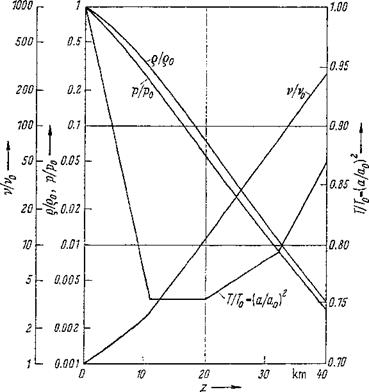Figure 1-2 Atmospheric pressure p, air density o, temperature T, speed of sound a, and kinematic viscosity v, vs. height z. From “U. S. Standard Atmosphere” [2].

is, therefore, a first important dimensionless characteristic number of flow processes. Since the effects of compressibility become noticeable for Ma> 0.3, as pointed out above, the Mach similarity law needs to be considered only above this limiting value. The fluid dynamic laws of an incompressible fluid can, therefore, be taken as the laws for very small Mach numbers with the limiting case Ma -> 0.

Reynolds similarity law Let us now consider the case of an incompressible, viscous flow. Here, only inertia and viscous forces act on the fluid element. These two forces are functions of the following physical quantities: approach velocity V, characteristic body dimension /, density q, and dynamic viscosity /x of the fluid. The only possible dimensionless combination of these quantities is the quotient

where Re is called the Reynolds number. The ratio ju/g = v has been introduced above in Eq. (1-7) as the kinematic viscosity. This law was found by Reynolds in 1883 during investigations on the flow in pipes and is called the Reynolds similarity law.

If velocity and body dimensions are not too small, as in aeronautics, the Reynolds number is very large because of the very small values of v. This means physically that the friction forces are much smaller than the inertia forces in such cases. Inviscid flow (y ->0) corresponds to the limiting case Re-*00. The laws of flow with small viscosity often correspond quite well to those without viscosity. On the other hand, in many cases even a very small viscosity should not be neglected in the theory (boundary-layer theory).

For compressible flow with friction, mechanical similarity requires that the Mach and Reynolds similarity laws be satisfied simultaneously, which is very difficult to accomplish in experimental investigations. The Mach similarity law and the Reynolds similarity law govern decisively the whole realm of theoretical and experimental fluid mechanics and particularly the laws of aeronautics.

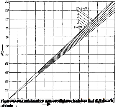
To give a convenient survey of the Mach and Reynolds numbers occurring in the aerodynamics of aircraft, the diagrams Fig. 1-3 and Fig. 1-4 have been drawn. They show these two dimensionless characteristic quantities versus flight velocity and flight altitude up to z = 20 km. Figure 1-3 shows that, at constant flight velocity, the Mach number increases with altitude because the sonic speed decreases, as was shown in Table 1-3. At an altitude of 10 km, the speed of sound has dropped to 300 m/s. At the same flight velocity, the Mach number at 10 km of altitude is about 10% larger than at sea level. This fact is important for the estimation of the aerodynamic properties of an airplane flying near the speed of sound.

The Reynolds numbers in Fig. 14 are those for a reference length of / = 1 m, where / may be the wing chord, fuselage length, or control surface chord. The Reynolds numbers of the diagram must be multiplied by a factor that corresponds to the reference length l in meters. Since the kinematic viscosity increases considerably with increasing height (see Table 1-3), the Reynolds number decreases

Figure 1-4 Reynolds number Re vs. flight velocity V and flight altitude 2.

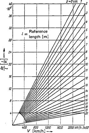
sharply with increasing height for a constant flight velocity, making airplane drag a particularly strong function of the height.

Changes of pressure, density, and viscosity of the air with altitude z of the stationary atmosphere are important for aeronautics. These quantities depend on the vertical temperature distribution T(z) in the atmosphere. At moderate altitude (up to about 10 km), the temperature decreases with increasing altitude, the temperature gradient dT/dz varying between approximately—0.5 and —1 К per 100 m, depending on the weather conditions. At the higher altitudes, the temperature gradient varies strongly with altitude, with both positive and negative values occurring.

The data for the atmosphere given below are valid up to the boundary of the homosphere at an altitude of about 90 km. Here the gravitational acceleration is already markedly smaller than at sea level.

The pressure change for a step of vertical height dz is, after the basic hydrostatic equation,

dp = —ggdz

ego d-H

where H is called scale height.

which shows that each polytropic exponent n belongs to a specific temperature gradient dT/dH. Note that the gas constant[1] in the homosphere, up to an altitude of H = 90 km, can be taken as a constant.

From Eq. (1-13) follows by integration:

T = T„ – (H – H„) (1-14)

Here it has been assumed that the polytropic exponent and, therefore, the temperature gradient are constant within a layer. The index b designates the values at the lower boundary of the layer. In Table 1-2 the values of Hb, zb, Tb, and dT/dH are listed according to the “U. S. Standard Atmosphere” [2].

The pressure distribution with altitude of the atmosphere is obtained through integration of Eq. (1-12д) with the help of Eq. (1-14). We have

For the special case n = 1 (isothermal atmosphere), Eq. (1-15д) reduces to

In the older literature this relationship is called the barometric height equation. Finally, the density distribution is easily found from the polytropic relation Eq. (1 -11*)-

Also given in Table 1-2 are the reference values pb and ob at the layer boundaries. For the bottom layer, which reaches from sea level to H~ 11 km, Hb = H0 has to be set equal to zero in Eqs. (1-15a) and (1-15£>). The other sea level values (index 0), inclusive of those for the speed of sound and the kinematic viscosity, are, after [2],

t0 = 15°C a0 = 340.29 m/s vQ = 1.4607 • 10’5 m2/s (dT/dH)о = -6.5 K/km

The numerical values of pressure and density distribution are listed in Table 1*3, to which the values for the speed of sound and the kinematic viscosity have been added. More detailed and more accurate values are found in the comprehensive tables [2].

Finally, in Fig. 1-2, a graphic representation is given of the distributions of pressure, density, temperature, speed of sound, and kinematic viscosity versus altitude. Whereas pressure and density decrease strongly with height, kinematic viscosity increases markedly.

1- І PROBLEMS OF AIRPLANE AERODYNAMICS

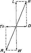
An airplane moves in the earth’s atmosphere. The state of motion of an airplane is determined by its weight, by the thrust of the power plant, and by the aerodynamic forces (or loads) that act on the airplane parts during their motion. For every state of motion at uniform velocity, the resultant of weight and thrust forces must be in equilibrium with the resultant of the aerodynamic forces. For the particularly simple state of motion of horizontal flight, the forces acting on the airplane are shown in Fig. 1-1. In this case, the equilibrium condition is reduced to the requirement that, in the vertical direction, the weight must be equal to the lift (W = L) and, in the horizontal direction, the thrust must be equal to the drag (Th =D). Here, lift L and drag D are the components of the aerodynamic force Rx normal and parallel, respectively, to the flight velocity vector V. For nonuniform motion of the aircraft, inertia forces are to be added to these forces.

In this book we shah deal exclusively with aerodynamic forces that act on the individual parts, and thus on the whole aircraft, during motion. The most important parts of the airplane that contribute to the aerodynamic forces are wing, fuselage, control and stabilizing surfaces (tail unit or empennage, ailerons, and canard surfaces), and power plant. The aerodynamic forces depend in a quite complicated manner on the geometry of these parts, the flight speed, and the physical properties of the air (e. g., density, viscosity). It is the object of the study of the aerodynamics of the airplane to furnish information about these interrelations. Here, the following two problem areas have to be considered:

1. Determination of aerodynamic forces for a given geometry of the aircraft (direct problem)

2. Determination of the geometry of the aircraft for desired flow patterns (indirect problem)

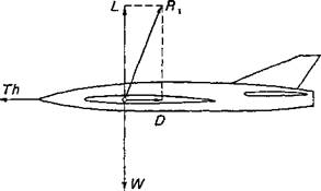Figure 1-1 Forces (loads) on an air­plane in horizontal flight. L, lift; D, drag; W, weight; Th, thrust; R1, re­sultant of aerodynamic forces (result­ant of L and D); R2, resultant of W and Th.

The object of flight mechanics is the determination of aircraft motion for given aerodynamic forces, known weight of the aircraft, and given thrust. This includes questions of both flight performance and flight conditions, such as control and stability of the aircraft. Flight mechanics is not a part of the problem area of this book. Also, the field of aeroelasticity, that is, the interactions of aerodynamic forces with elastic forces during deformation of aircraft parts, will not be treated.

The science of the aerodynamic forces of airplanes, to be treated here, forms the foundation for both flight mechanics and many questions of aircraft design and construction.

1- 2-1 Basic Facts

In fluid mechanics, some physical properties of the fluid are important, for example, density and viscosity. With regard to aircraft operation in the atmosphere, changes of these properties with altitude are of particular importance. These physical properties of the earth’s atmosphere directly influence aircraft aero­dynamics and consequently, indirectly, the flight mechanics. In the following discussions the fluid will be considered to be a continuum.

The density q is defined as the mass of the unit volume. It depends on both pressure and temperature. Compressibility is a measure of the degree to which a fluid can be compressed under the influence of external pressure forces. The compressibility of gases is much greater than that of liquids. Compressibility

therefore has to be taken into account when changes in pressure resulting from a particular flow process lead to noticeable changes in density.

Viscosity is related to the friction forces within a streaming fluid, that is, to the tangential forces transmitted between ambient volume elements. The viscosity coefficient of fluids changes rather drastically with temperature.

In many technical applications, viscous forces can be neglected in order to simplify the laws of fluid dynamics (inviscid flow). This is done in the theory of lift of airfoils (potential flow). To determine the drag of bodies, however, the viscosity has to be considered (boundary-layer theory). The considerable increase in flight speed during the past decades has led to problems in aircraft aerodynamics that require inclusion of the compressibility of the air and often, simultaneously, the viscosity. This is the case when the flight speed becomes comparable to the speed of sound (gas dynamics). Furthermore, the dependence of the physical properties of air on the altitude must be known. Some quantitative data will now be given for density, compressibility, and viscosity of air. Material Properties

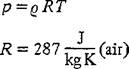
Density The density of a gas (mass/volume), with the dimensions kg/m3 or Ns2/m4, depends on pressure and temperature. The relationship between density q, pressure p, and absolute temperature T is given by the thermal equation of state for ideal gases

(l-lc)

(1-1£) where R is the gas constant. Of the various possible changes of state of a gas, of particular importance is the adiabatic-reversible (isentropic) change in which pressure and density are related by

P

— = const

Here 7 is the isentropic exponent, with

(1-Зя)

= 1.405 (air)

cp and cv are the specific heats at constant pressure and constant volume, respectively.

Very fast changes of state are adiabatic processes in very good approximation, because heat exchange with the ambient fluid elements is relatively slow and, therefore, of negligible influence on the process. In this sense, dow processes at high speeds can usually be considered to be fast changes of state. If such flows are steady, isentropic changes of state after Eq. (1-2) can be assumed. Unsteady-flow

processes (e. g., with shock waves) are not isentropic (anisentropic); they do not follow Eq. (1-2).

Across a normal compression shock, pressure and density are related by

(7-1)+ (7+ 1) —

(h _____________________ El

Qi Pt

(7 + 1) + (7 — l)~r Pi

7+1

<-—r = 5.93 (air)

7 — I v ‘

where the indices 1 and 2 indicate conditions before and behind the shock, respectively.

Speed of sound Since the pressure changes of acoustic vibrations in air are of such a high frequency that heat exchange with the ambient fluid elements is negligible, an isentropic change of state after Eq. (1-2) can be assumed for the compressibility law of air: p{q). Then, with Laplace’s formula, the speed of sound becomes

a = ]/7 RT 0‘5fl)

a0 = 340 m/s (air) (1 -5 b)

where for pie the value given by the’ equation of state for ideal gases, Eq. (1-lar), was taken. Note that the speed of sound is simply proportional to the square root of the absolute temperature. The value given in Eq. (1 -5b?) is valid for air of temperature t = 15°C or T = 288 K.

Viscosity In flows of an inviscid fluid, no tangential forces (shear stresses) exist between ambient layers. Only normal forces (pressures) act on the flow. The theory of inviscid, incompressible flow has been developed mathematically in detail, giving, in many cases, a satisfactory description of the actual flow, for example, in computing airfoil lift at moderate flight velocities. On the other hand, this theory fails completely for the computation of body drag. This unacceptable result of the theory of inviscid flow is caused by the fact that both between the layers within the fluid and between the fluid and its solid boundary, tangential forces are transmitted that affect the flow in addition to the normal forces. These tangential or friction forces of a real fluid are the result of a fluid property, called the viscosity of the fluid. Viscosity is defined by Newton’s elementary friction law of fluids as

du

T=^

Here 7 is the shearing stress between adjacent layers, dujdy is the velocity gradient nor­mal to the stream, and д is the dynamic viscosity of the fluid, having the dimensions Ns/m2. It is a material constant that is almost independent of pressure but, in gases,
increases strongly with increasing temperature. In all flows governed by friction and inertia forces simultaneously, the quotient of viscosity p and density g plays an important role. It is called the kinematic viscosity v, and has the dimensions m2/s. In Table 1-1 a few values for density o, dynamic viscosity ju, and kinematic viscosity v of air are given versus temperature at constant pressure.

Only a very few comprehensive presentations of the scientific fundamentals of the aerodynamics of the airplane have ever been published. The present book is an English translation of the two-volume work “Aerodynamik des Flugzeuges,” which has already appeared in a second edition in the original German. In this book we treat exclusively the aerodynamic forces that act on airplane components—and thus on the whole airplane—during its motion through the earth’s atmosphere (aerodynamics of the airframe). These aerodynamic forces depend in a quite complex manner on the geometry, speed, and motion of the airplane and on the properties of air. The determination of these relationships is the object of the study of the aerodynamics of the airplane. Moreover, these relationships provide the absolutely necessary basis for determining the flight mechanics and many questions of the structural requirements of the airplane, and thus for airplane design. The aerodynamic problems related to airplane propulsion (power plant aerodynamics) and the theory of the modes of motion of the airplane (flight mechanics) are not treated in this book.

The study of the aerodynamics of the airplane requires a thorough knowledge of aerodynamic theory. Therefore, it was necessary to include in the German edition a rather comprehensive outline of fluid mechanic theory. In the English edition this section has been eliminated because there exist a sufficient number of pertinent works in English on the fundamentals of fluid mechanic theory.

Chapter 1 serves as an introduction. It describes the physical properties of air and of the atmosphere, and outlines the basic aerodynamic behavior of the airplane. The main portion of the book consists of three major divisions. In the first division (Part 1), Chaps. 2-4 cover the aerodynamics of the airfoil. In the second division (Part 2), Chaps. 5 and 6 consider the aerodynamics of the fuselage and of the wing-fuselage system. Finally, in the third division (Part 3), Chaps. 7 and 8 are devoted to the problems of the aerodynamics of the stability and control systems (empennage, flaps, and control surfaces). In Parts 2 and 3, the interactions among the individual parts of the airplane, that is, the aerodynamic interference, are given special attention.

Specifically, the following brief outline describes the chapters that deal with the intrinsic problems of the aerodynamics of the airplane: Part 1 contains, in Chap. 2, the profile theory of incompressible flow, including the influence of friction on the profile

characteristics. Chapter 3 gives a comprehensive account of three-dimensional wing theory for incompressible flow (lifting-line and lifting-surface theory). In addition to linear airfoil theory, nonlinear wing theory is treated because it is of particular importance for modem airplanes (slender wings). The theory for incompressible flow is important not only in the range of moderate flight velocities, at which the compressibility of the air may be disregarded, but even at higher velocities, up to the speed of sound—that is, at all Mach numbers lower than unity—the pressure distribution of the wings can be related to that for incompressible flow by means of the Prandtl-Glauert transformation. In Chap. 4, the wing in compressible flow is treated. Here, in addition to profile theory, the theory of the wing of finite span is discussed at some length. The chapter is subdivided into the aerodynamics of the wing at subsonic and supersonic, and at transonic and hypersonic incident flow. The latter two cases are treated only briefly. Results of systematic experimental studies on simple wing forms in the subsonic, transonic, and supersonic ranges are given for the qualification of the theoretical results. Part 2 begins in Chap. 5 with the aerodynamics of the fuselage without interference at subsonic and supersonic speeds. In Chap. 6, a rather comprehensive account is given of the quite complex, but for practical cases very important, aerodynamic interference of wing and fuselage (wing-fuselage system). It should be noted that the difficult and complex theory of supersonic flow could be treated only superficially. In this chapter, a special section is devoted to slender flight articles. Here, some recent experimental results, particularly for slender wing-fuselage systems, are reported. In Part 3, Chaps. 7 and 8, the aerodynamic questions of importance to airplane stability and control are treated. Here, the aerodynamic interferences of wing and wing-fuselage systems are of decisive significance. Experimental results on the maximum lift and the effect of landing flaps (air brakes) are given. The discussions of this part of the aerodynamics of the airplane refer again to subsonic and supersonic incident flow.

A comprehensive list of references complements each chapter. These lists, as well as the bibliography at the end of the book, have been updated from the German edition to include the most recent publications.

Although the book is addressed primarily to students of aeronautics, it has been written as well with the engineers and scientists in mind who work in the aircraft industry and who do research in this field. We have endeavored to emphasize the theoretical approach to the problems, but we have tried to do this in a manner easily understandable to the engineer. Actually, through proper application of the laws of modern aerodynamics it is possible today to derive a major portion of the aerodynamics of the airplane from purely theoretical considerations. The very comprehensive experimental material, available in the literature, has been included only as far as necessary to create a better physical concept and to check the theory. We wanted to emphasize that decisive progress has been made not through accumulation of large numbers of experimental results, but rather through synthesis of theoretical considerations with a few basic experimental results. Through numerous detailed examples, we have endeavored to enhance the reader’s comprehension of the theory.

Hermann Schlichting Erich Truckenbrodt