Our heavyweight helicopter equal in the world does not have
In Rostov started production of the most load-lifting rotary-wing car The Russian holding «Helicopt[...]

Everything about aircrafts and helicopters. News and events in aviation worldwide. Civil, transportation, military helicopters and airplanes.

Everything about aircrafts and helicopters. News and events in aviation worldwide. Civil, transportation, military helicopters and airplanes.

Everything about aircrafts and helicopters. News and events in aviation worldwide. Civil, transportation, military helicopters and airplanes.

Everything about aircrafts and helicopters. News and events in aviation worldwide. Civil, transportation, military helicopters and airplanes.


2- 4-1 Singularities
The method of conformal mapping was applied in Sec. 2-3 to the computation of velocity distributions about a given wing profile. Another means of computing the aerodynamic properties of wing profiles is the method of singularities (see Keune and Burg [33]). This consists of arranging sources, sinks, and vortices within the profile. Through superposition of their flow fields with a translational flow, a suitable body contour (profile) is produced. The flow field within the contour has no physical meaning. For the creation of a symmetric profile in a symmetric incident flow field (teardrop profile), only sources and sinks are required, whereas for the creation of camber, vortices must be added within the profile. This procedure is shown schematically in Fig. 2-19.
These sources, sinks, and vortices are termed singularities of the flow. In most cases it is necessary to distribute the singularities continuously over the profile chord rather than discretely.
It is expedient to treat the very thin profile (skeleton profile) first. For such profiles the skeleton theory (Sec. 24-2) produces all essential results for their lift. For representation of the skeleton profile, only a vortex distribution is needed. The symmetric profile of finite thickness (teardrop profile) in symmetric flow (angle of attack zero) is produced by source-sink distributions (teardrop theory). In this case the displacement flow about the profile is obtained (Sec. 24-3). The cambered
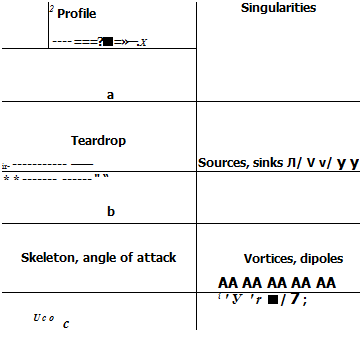 Figure 2-19 The singularities method. (a) Cambered profile of finite thickness with angle of attack а. (&) Symmetric profile of finite thickness in symmetric flow, a = 0. (c) Very thin profile with angle of attack.
![]()
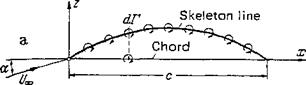
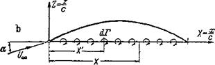
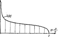 Figure 2-20 The skeleton theory. (a) Arrangement of the vortex distribution on the skeleton line, (b) Arrangement of the vortex distribution on the chord (slightly cambered profile), (c) Circulation distribution along the chord (schematic).
profile of finite thickness is essentially the product of superposition of a mean camber line (skeleton line) with a teardrop profile (Sec. 24-4).
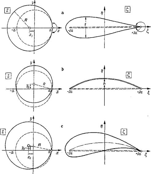
The Joukowsky transformation (mapping) function Eq. (2-21) is also particularly suitable for the generation of thick and cambered profiles. In Sec. 2-3-1 it was shown that this transformation function maps the circle z = a about the origin in the z plane into the straight line f = —2a to f = +2a of the £ plane (Fig. 2-8g).
The same transformation function also allows generation of body shapes resembling airfoils by choosing different circles in the z plane. These shapes may have rounded noses and sharp trailing edges (Fig. 2-14). They are called Joukowsky profiles, after which the transformation function is named. By choosing a circle in the 2 plane as in Fig. 2-14a, the center of which is shifted by x0 on the negative axis from that of the unit circle and which passes through the point z = a, a profile is produced that resembles a symmetric airfoil shape. It encircles the slit from —2a to +2a. This is a symmetric Joukowsky profile, the thickness t of which is determined by the location x0 of the center of the mapping circle. The profile tapers toward the trailing edge with an edge angle of zero.
Circular-arc profiles are obtained when the center of the mapping circle lies on the imaginary axis (Fig. 2-14h). When the center is set on +iy0 and the circumference passes through z — +a, the same mapping function produces a
|
Figure 2-14 Generation of Joukowsky profiles through conformal mapping with the Joukowsky mapping function, Eq. (2-21). (a) Symmetric Joukowsky profile, {b) Circular-arc profile, (c) Cambered Joukowsky profile. |
twice-passed circular arc in the £ plane. It lies between £=—2a and f = +2a. The height h of this circular arc depends on y0. Finally, by choosing a mapping circle the center of which is shifted both in the real and the imaginary directions (Fig.
2- 14c), a cambered Joukowsky profile is mapped, the thickness and camber of which are determined by the parameters x0 and yQ, respectively.
As a special case of the Joukowsky profiles, the very thin circular-arc profile (circular-arc mean camber) will be discussed.
Circular-arc profile In the circular-arc profile the mapping circle in the z plane is a circle, as in Fig. 2-14b, passing through the points z = Л-а and z = —a with its center at a distance y0 from the origin on the imaginary axis. The radius of the mapping circle is R = ayl + є? with ej = y0/a. The circle К is mapped into a twice-passed
profile in the £ plane, extending from f = —2a to £ = +2a. This profile has a chord length c = 4a and a camber height hja = 2ех, or
h 1
-7 = ^ (2-34)
It is easily shown that the profile in the f plane is a portion of a circle for any єі. For small camber (є? ^ 1), the profile contour is given by
![]() (2-35)
(2-35)
This profile is also called a parabola skeleton. For small angles of attack, a< 1, and small camber, the lift coefficient becomes
The lift slope dcildoi. is again equal to 2tt for small angles of attack, as in the case of the inclined flat plate according to Eq. (2-31). For the zero-lift angle of attack this equation yields a0 = —2(h/c). The pitching-moment coefficient about the profile leading edge becomes
см=-|(а + 41) (2-37)
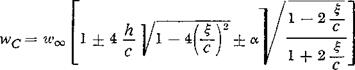
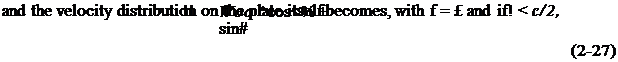
resulting in смо = —Tc(h/c) for the zero-moment coefficient whena0 = —2(hfc). The velocity distribution on the circular-arc profile is given for small camber and small angles of attack by
 (2-38)
The + sign applies to the upper profile surface, the — sign to the lower profile surface. The second term, which is dependent on the camber, represents an elliptic distribution over %. The third term, which depends on the angle of attack a, corresponds to the expression found for the inclined flat plate [Eq. (2-27)].
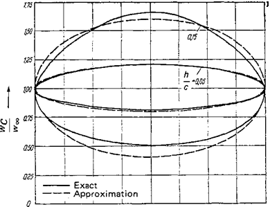
At the trailing edge, % = cj2, the velocity on the circular-arc profile is finite, whereas in general its value becomes infinitely large at the leading edge, = — c/2. Only for the angle of incidence a = 0 does the velocity remain finite at the leading edge. This is the angle of smooth leading-edge flow (no flow around the leading edge).* Velocity distributions, computed for this case, are shown in Fig. 2-15 for
Translator’s note: When the angle of attack of a thin profile (skeleton) is changed from positive to negative values, the stagnation point moves from the lower surface to the upper surface. Only at one angle of attack is the stagnation point exactly on the leading edge. This angle is called the angle of smooth leading-edge flow (S. L.E. F.). Obviously, here, no flow rounds the leading edge, which-in inviscid flow-would cause infinitely high velocities. Rather, the S. L.E. F. is a smooth flow past the leading edge. Only for a flat plate is the angle of S. L.E. F. equal to the angle of attack a = 0.
 |
 |
two circular-arc profiles of camber hjc — 0.05 and 0.15. For comparison, the exactly computed distributions are also given. The agreement is very good for small camber. For larger camber, some deviations can be seen.
Of particular interest is the largest velocity on the profile at a = 0. It occurs at the profile center | = 0 and is obtained from Eq. (2-38) as
WCmax = vv„^l+4^ (2-39a)
= (2-39&)
These equations allow a very simple estimation of the maximum velocity on a very thin circular-arc profile with smooth leading-edge flow.
Inclined symmetric Joukowsky profile The symmetric Joukowsky profile may serve as a further example. This profile is obtained from Fig. 2-14a when the mapping circle passes through the point z — 4-а and is placed with its center on the negative real axis at a distance x0 from the origin. The radius of the circle is
R = a + x0 = а(1 + e2) with є2 = ~ (240)
The unit circle and the mapping circle are tangent in z = a; that is, the tangents of the two circles intersect under the angle zero. Since the angles remain unchanged in conformal mapping, the trailing-edge angle of the Joukowsky profile is zero.[6] For a
very small thickness {z < 1), the profile chord length is c = 4a and the thickness
![]() ^=|V3e2 = 1.299E2
^=|V3e2 = 1.299E2
The maximum thickness occurs at </?= 120°, that is, at point c/4 from the leading edge. The profile contour is given by
![]() (242)
(242)
This profile shape is called the Joukowsky teardrop. The zero-lift direction of this profile coincides with the profile chord (the £ axis).
The lift coefficient is

cL = 27г(1 + e2) sin a
where the second expression is valid for small angles of attack. Accordingly, the lift slope dcLjdoc increases somewhat with profile thickness.
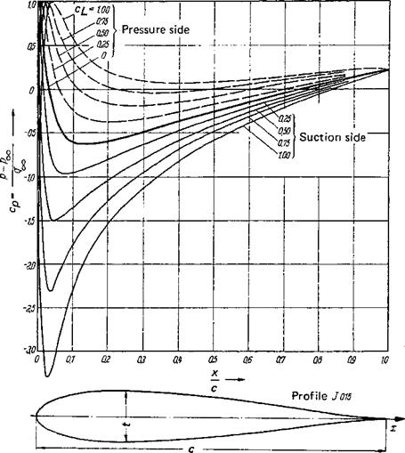
The pitching-moment coefficient about the profile leading edge becomes cm ~~(rr/2)(l +£2)0, indicating that the lift force center of attack (neutral point) lies at a distance c/4 from the profile nose. The velocity distribution on the contour of the symmetric Joukowsky profile is obtained in a way similar to that for the circular-arc profile. Presentation of the corresponding expression is omitted. In Fig.
2- 16, pressure distributions on a symmetric Joukowsky profile of 15% thickness ratio are presented for various lift coefficients. At an angle of attack a = 0 (c^ — 0), the pressure minimum occurs at approximately 15% chord behind the nose. When the angle of attack increases, the minimum moves forward on the suction side and farther back on the pressure side.
Cambered Joukowsky profiles The Joukowsky profile with a mean camber line shaped like a circular arc is obtained by mapping an excentrically located circle with its center at z0 = x0 + iy0 (see Fig. 2-14c). Further generalizations of the Joukowsky mapping functions are given by von Karman and Trefftz [7], with profile thickness, camber height, and trailing-edge angle as the parameters. The mean camber line has the shape of a circular arc, however, as in the case of the Joukowsky profiles, resulting in a considerable shift of the aerodynamic center. For the elimination of this problem, Betz and Keune [7] developed suitable mapping functions.
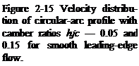
Experimental results Comprehensive three-component measurements on numerous Joukowsky profiles have been reported in [47]. Figure 2-17 shows a comparison of lift coefficients versus the angle of attack as obtained from theory and tests by Betz [31]. The agreement is quite good in the angle-of-attack range from a =—10° to
|
Figure 2-16 Pressure distribution of an inclined symmetric Joukowsky profile, t/c = 0.15, for various lift coefficients c^. |
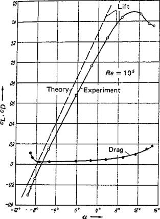
a = +10°; the small differences are caused by viscous effects. The moment curves cm(cl) are i*1 agreement with theory up to large thickness ratios in the case of symmetric profiles; in the case of cambered profiles, however, the agreement is good only for small thickness ratios. The theoretical and experimental pressure distributions are also in good agreement, as can be seen from Fig, 2-18.
Concluding remarks The disadvantage of using the method of conformal mapping to determine aerodynamic properties of profiles lies in the necessity of first finding a mapping function. The resulting profile shape must then be compared with the desired shape. In general, it is not possible to know beforehand the proper mapping function that is mapping the desired profile shape on the circle. To a first approximation, this problem can be solved as shown by Theodorsen and Garrick [66]; see also Ringleb [32]. The methods for the treatment of profile theory by means of conformal mapping will not be discussed further, because the method of singularities, which will be discussed next, has proved to be more suitable and allows simpler computation of velocity distributions over a given profile. Furthermore, the method of singularities has the marked advantage over the method of
Figure 2-17 Lift and drag for plane flow around a cambered Joukowsky profile, after Betz [31]. Profile after Fig. 2-18.
 conformal mapping that it can be applied to three-dimensional problems (wings of finite span) whereas conformal mapping is strictly limited to two-dimensional problems. The great value of the method of conformal mapping remains nevertheless, because this method allows one to establish exact solutions for the velocity distribution on certain profiles that then can be compared with approximate solutions as obtained, for instance, by the method of singularities. For the design
 Figure 2-18 Comparison of theoretical and experimental pressure distributions of an inclined cambered Joukowsky profile resulting in the same lift, after Betz [31].
problem, that is, the problem of determining the profile shape for a given pressure distribution, Eppler [13] has developed a procedure that uses conformal mapping.
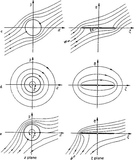
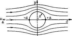
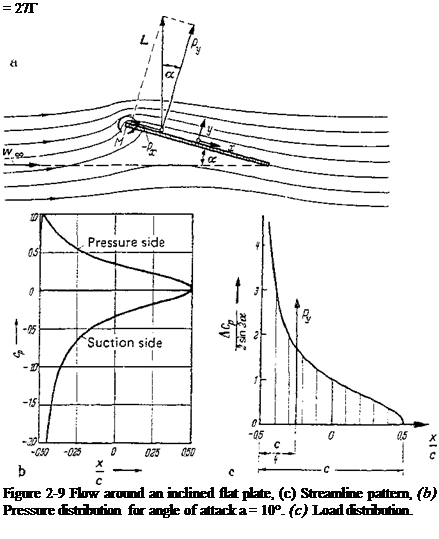
The simplest case of a lifting-airfoil profile is the inclined flat plate. The angle between the direction of the incident flow and the direction of the plate is called angle of attack a of the plate.
The flow about the inclined flat plate is obtained as shown in Fig. 2-8, by superposition of the plate in parallel flow (a) and the plate in normal flow (b). The resulting flow
(c) = (a) + (b)
does not yet produce lift on the plate because identical flow conditions exist at the leading and trailing edges. The front stagnation point is located on the lower surface and the rear stagnation point on the upper surface of the plate.
|
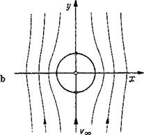
To establish a plate flow with lift, a circulation Г according to Fig. 2-М must be superimposed on (c). The resulting flow
0) = (c) + (d) = (a) + (b) + (d)
is the plate flow with lift. The magnitude of the circulation is determined by the condition of smooth flow-off at the plate trailing edge; for example, the rear stagnation point lies on the plate trailing edge (Kutta condition). By superposition of the three flow fields, a flow is obtained around the circle of radius a with its center at z = 0. It is approached by the flow under the angle a with the jc axis, a being arctan (v^/Uoo). The complex stream function of this flow, taking Eqs. (2-18) and (2-19) into account, becomes
F(z) — (Uoo — і Voo) z + (««, – j – г Vcc) 4- + т£іпг (2-24)
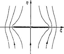
For the mapping, the Joukowsky transformation function from Eq. (2-21) was chosen. This function transforms the circle of radius a in the z plane into the plate of length c = 4a in the f plane. The velocity distribution about the plate is obtained with the help of Eq. (2-23) after some auxiliary calculations as
00 ъ o-r
= (2-25)
The magnitude of the circulation Г is now to be determined from the Kutta condition. Smooth flow-off at the trailing edge requires that there—that is, at $ = +2л—the velocity remains finite. Therefore, the nominator of the fraction in Eq. (2-25) must vanish for f = 2a. Hence, because of 4a — c,

 |
Г = 47raUoo = rtcvaо
The + sign applies to the upper surface, the — sign to the lower surface. With w«, the resultant of the incident flow, and a, the angle of attack between plate and incident flow resultant, the flow components are given by = w«, cos a and vx = sin a.
At the plate leading edge, f = —c/2, the velocity is infinitely high. The flow around the plate comes from below, as seen from Fig. 2-8c. On the plate trailing edge, f = 4-е/2, the tangential velocity has the value u = vm cos a. At an arbitrary station of the plate, the tangential velocities on the lower and upper surfaces have a difference in magnitude Ли = uu —щ. At the trailing edge, Л и = 0 (smooth flow-off). The nondimensional pressure difference between the lower and upper surfaces, related to the dynamic pressure of the incident flow qx = (o/2)wi, is [see Eq. (2-8)]
 |
where uu and щ stand for the velocities on the upper and lower surfaces of the plate, respectively. This load distribution on the plate chord is demonstrated in Fig. 2-9c. The loading at the plate leading edge is infinitely large, whereas it is zero at the trailing edge. By integration, the force resulting from the pressure distribution on the surface can he computed in principle [see Eq. (2-9)]. In the present case, the result is obtained more simply by introducing Eq. (2-266) into Eq. (2-15). With
L = QTtbcwl, sin a (2-29)
the lift coefficient becomes
This equation establishes the basic relationship between the lift coefficient and the angle of attack of a flat plate in two-dimensional flow. The so-called lift slope for small a is
![]()
dcL
da
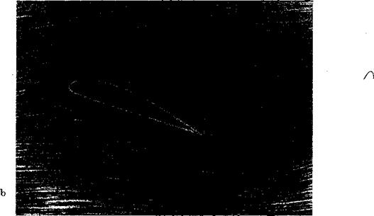
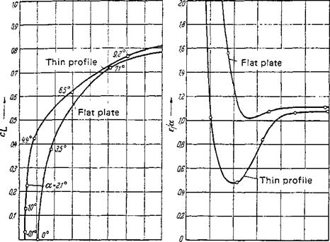
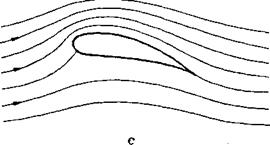
Figure 2-10 gives a comparison, based on Eq. (2-30), between theory and experimental measurements for a flat plate and a very thin symmetric profile. Up to about a-6°, the agreement is quite good, although it is somewhat better for the plate than for the profile. At angles of attack in excess of 8°, the experimental curves lie considerably below the theoretical curve, a deviation due to the effect of viscosity. When the angle of attack exceeds 12°, flow separation sets in. Flows around profiles with and without separation are shown in Fig. 2-11. Naumann [42] reports measurements on a profile over the total possible range of angle of attack, that is, for 0° < a < 3’60°.
Without derivation, the pitching moment coefficient about the plate leading edge (tail-heavy taken to be positive) is given by
cm = —f— = — x sin2i* (2-32)
bc*q0о *
From Eqs. (2-30) and (2-32), the distance of the lift center of application from the leading edge at small angles of attack is obtained (see Fig. 2-9) as
![]() _ _£M = 1
_ _£M = 1
C CL 4
Since lift and moment depend exclusively on the angle of attack, the center of lift (= center of application of the load distribution in Fig. 2-9c) is identical to the neutral point (see Sec. 1-3-3).
An astounding result of the just computed inviscid flow about an infinitely thin
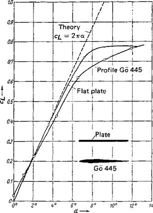 Figure 2-10 Lift coefficient vs. angle of attack a for a flat plate and a thin symmetric profile. Comparison of theory, Eq. (2-30), and experimental measurements, after Prandtl and Wieselsberger [47].
|
|
|
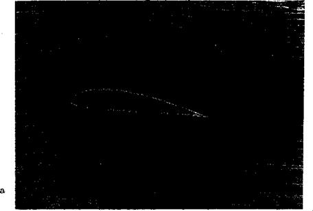
Figure 2-11 Photographs of the flow about airfoil, after Prandtl and Wieselsberger [47]. (a) Attached flow. (b) Separated flow. |
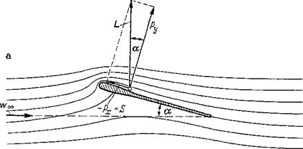
inclined flat plate is the fact that the resultant L of the forces is not perpendicular to the plate, but perpendicular to the direction of the incident flow (Fig. 2-9a). Since only normal forces (pressures) are present on the plate surface in a frictionless flow, it could appear to be likely that the resultant of the forces acts normal to the plate, too. Besides the normal component Py=Lcosa, however, there is a tangential component Px = —L sin a that impinges on the plate leading edge. Together with the normal component Py, the resultant force L acts normal to the direction of the incident flow. For the explanation of the existence of a tangential component Px in an inviscid flow—we shall call it suction force—a closer look at the flow process is required. The suction force has to do with the flow at the plate nose, which has an infinitely high velocity. Consequently, an infinitely high underpressure is produced. This condition is easier to see in the case of a plate of finite but small thickness and rounded nose (Fig. 2-12a). Here the underpressure at the nose of the plate is finite and adds up to a suction force acting parallel to the plate in the forward direction. The detailed computation shows that the magnitude of this suction force is independent of plate thickness and nose rounding. It remains, therefore, the value of S = L sin a in the limiting case of an infinitely thin plate.
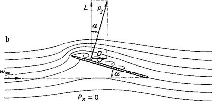
In real flow (with friction) around very sharp-nosed plates, an infinitely high underpressure does not exist. Instead, a slight separation of the flow (separation bubble) forms near the nose (Fig. 2-12b). For small angles of attack, the flow reattaches itself farther downstream and, therefore, on the whole is equal to the frictionless flow. The suction force is missing, however, and the real flow around an inclined sharp-edged plate produces drag acting in the direction of the incident flow. Also, this analysis shows that it is very important for keeping the drag small that the leading edge of wing profiles is well rounded. Figure 2-13 shows (a) the polar curves (cL vs. Cq) and (b) the glide angles e= cDjcL of a thin sharp-edged flat plate and of a thin symmetric profile. In the range of small to moderate angles of attack, the thin profile with rounded nose has a markedly smaller drag than the sharp-edged flat plate. Within a certain range of angles of attack, є is smaller than а (є < a) for
|
|
|
Figure 2-12 Development of the suction force S on the leading edge of a profile, (a) Thin, symmetric profile with rounded nose, suction force present. (b) Flat plate with sharp nose, suction force missing. |
|
0 0,02 0№ 0.06 008 010 0.12 № 0.16 0° 2° <t° 6° 8° !0° 12° a CQ —► b a ^ Figure 2-13 Aerodynamic coefficients of a sharp-edged flat plate and a thin symmetric profile for Re = 4′ 10s, A = », from Prandtl and Wieselsberger [47]. {a) Polar curves, vs. cjj. (Ъ) Glide angle, є = cd/cd- |
thin profiles; the resultant of the aerodynamic forces is inclined upstream relative to the direction normal to the profile chord. This must be attributed to the effect of the suction force.
2- 3-1 Complex Presentation
Complex stream function Computation of a plane inviscid flow requires much less effort than that of three-dimensional flow. The reason lies not so much in the fact that the plane flow has only two, instead of three, local coordinates as that it can be treated by means of analytical functions. This is a mathematical discipline, developed in great detail, in which the two local coordinates (x, у) of two-dimensional flow can be combined to a complex argument. A plane, frictionless, and incompressible flow can, therefore, be represented as an analytical function of the complex argument z = x + iy:
F{z) = F{x + iy) = Ф(х, у) + і ¥{x, у) (2-16)
where Ф and У7, the potential and stream functions, are real functions of x and y. The curves Ф = const (potential lines) and lF = const (streamlines) form two families of orthogonal curves in the xy plane. By taking a suitable streamline as a solid wall, the other streamlines then form the flow field above this wall. The velocity components in the x and у directions, that is, и and v, are given by
_ дФ _ dW _ дФ _ 0 XF
U dx dy V dy Ox
The function F(z) is called a complex stream function. From this function, the velocity field is obtained immediately by differentiation in the complex plane, where
— = u —iv= vv(z) (2-17)
Here, w = u—iv is the conjugate complex number to w—uFiv, which is obtained by reflection of w on the real axis. In words, Eq. (2-17) says that the derivative of the complex stream function with respect to the argument is equal to the velocity vector reflected on the real axis.
The superposition principle is valid for the complex stream function precisely as for the potential and stream functions, because F(z’)= c1Fi(z) + c2F2(z) can be considered to be a complex stream function as well as F1(z’) and F2(z).
For a circular cylinder of radius a, approached in the x direction by the undisturbed flow velocity u00, the complex stream function is
F{z)=uO0(z + ^j (2-18)
For an irrotational flow around the coordinate origin, that is, for a plane potential vortex, the stream function is
*■<*) = (2-19)
where Г is a clockwise-turning circulation.
Conformal mapping First, the term conformal mapping shall be explained (see [6]). Consider an analytical function of complex variables and split it into real and imaginary components:
/(2) = IH І У) = С = £ (Ж, у) + і V (х> у) (2-20)
The relationship between the complex numbers z = x 4- iy and f = % + irj in Eq. (2-20) can be interpreted purely geometrically. To each point of the complex z plane a point is coordinated in the f plane that can be designated as the mirror image of the point in the z plane. Specifically, when the point in the z plane moves along a curve, the corresponding mirror image moves along a curve in the f plane. This curve is called the image curve to the curve in the z plane. The technical expression of this process is that, through Eq. (2-20), the z plane is conformally mapped on the £ plane. The best known and simplest mapping function is the Joukowsky mapping function,
![]() (2-21)
(2-21)
It maps a circle of radius a about the origin of the z plane into the twice-passed straight line (slit) from -2a to +2a in the f plane.
For the computation of flows, this purely geometrical process of conformal mapping of two planes on each other can also be interpreted as transforming a certain system of potential lines and streamlines of one plane into a system of those in another plane. The problem of computing the flow about a given body can then be solved as follows. Let the flow be known about a body with a contour A in the z plane and its stream function F(z), for which, usually, flow about a circular cylinder is assumed [see Eq. (2-18)]. Then, for the body with contour В in the f plane, the flow field is to be determined. For this purpose, a mapping function
£ = /(*) (2-22)
must be found that maps the contour A of the z plane into the contour В in the f plane. At the same time, the known system of potential lines and streamlines about the body A in the z plane is being transformed into the sought system of potential lines and streamlines about the body В in the f plane. The velocity field of the body В to be determined in the f plane is found from the formula
F(z) and w(z) are known from the stream function of the body A in the z plane (e. g., circular cylinder). Here dz/a= 1 jfz) is the reciprocal differential quotient of the mapping function f = /(z). The sought velocity distribution about body В can be computed from Eq. (2-23) after the mapping function /(z) that maps body A into body В has been found. The computation of examples shows that the major task of this method lies in the determination of the mapping function f = f(z), which maps the given body into another one, the flow of which is known (e. g., circular cylinder).
Applying the method of complex functions, von Mises [71] presents integral formulas for the computation of the force and moment resultants on wing profiles in frictionless flow. They are based on the work of Blasius [71].
Since the Kutta-Joukowsky equation (Eq. 2-15), which forms the basis of lift theory, has been introduced, the computation of lift can now be discussed in more detail. First, the two-dimensional problem will be treated exclusively, that is, the airfoil of infinite span in incompressible flow. The theory of the airfoil of infinite span is also called profile theory. Comprehensive discussions of incompressible profile theory, taking into account nonlinear effects and friction, are given by Betz [5], von Karman and Burgers [70], Sears [59], Hess and Smith [23], Robinson and Laurmann [51], Woods [74], and Thwaites [67]. A comparison of results of profile theory with measurements was made by Hoerner and Borst [25], Riegels [50], and Abbott and von Doenhoff [1].
Profile theory can be treated in two different ways (compare [73]): first, by the method of conformal mapping, and second, by the so-called method of singularities. The first method is limited to two-dimensional problems. The flow about a given body is obtained by using conformal mapping to transform it into a known flow about another body (usually circular cylinder). In the method of singularities, the body in the flow field is substituted by sources, sinks, and vortices, the so-called singularities. The latter method can also be applied to three – dimensional flows, such as wings of finite span and fuselages. For practical purposes, the method of singularities is considerably simpler than conformal mapping. The method of singularities produces, in general, only approximate solutions, whereas conformal mapping leads to exact solutions, although these often require considerable effort.
If the magnitude of the circulation is known, the Kutta-Joukowsky formula, Eq. (2-15), is of practical value for the calculation of lift. However, it must be clarified as to what way the circulation is related to the geometry of the wing profile, to the velocity of the incident flow, and to the angle of attack. This interrelation cannot be determined uniquely from theoretical considerations, so it is necessary to look for empirical results.
The technically most important wing profiles have, in general, a more or less sharp trailing edge. Then the magnitude of the circulation can be derived from experience, namely, that there is no flow around the trailing edge, but that the fluid flows off the trailing edge smoothly. This is the important Kutta flow-off condition, often just called the Kutta condition.
For a wing with angle of attack, yet without circulation (see Fig. 2-6a), the rear stagnation point, that is, the point at which the streamlines from the upper and lower sides recoalesce, would lie on the upper surface. Such a flow pattern would be possible only if there were flow around the trailing edge from the lower to the upper surface and, therefore, theoretically (in inviscid flow) an infinitely high velocity at the trailing edge with an infinitely high negative pressure. On the other hand, in the case of a very large circulation (see Fig. 2-6b) the rear stagnation point would be on the lower surface of the wing with flow around the trailing edge from above. Again velocity and negative pressure would be infinitely high.
Experience shows that neither case can be realized; rather, as shown in Fig.
2- 6c, a circulation forms of the magnitude that is necessary to place the rear stagnation point exactly on the sharp trailing edge. Therefore, no flow around the trailing edge occurs, either from above or from below, and smooth flow-off is established. The condition of smooth flow-off allows unique determination of the magnitude of the circulation for bodies with a sharp trading edge from the body shape and the inclination of the body relative to the incident flow direction. This statement is valid for the inviscid potential flow. In flow with friction, a certain reduction of the circulation from the value determined for frictionless flow is observed as a result of viscosity effects.
For the formation of circulation around a wing, information is obtained from
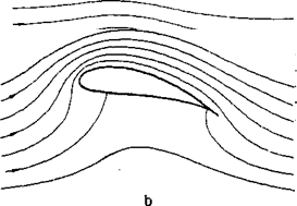 |
Figure 2-6 Flow around an airfoil for various values of circulation, (a) Circulation Г= 0: rear stagnation point on upper surface. (b) Very large circulation: rear stagnation point on lower surface. (c) Circulation just sufficient to put rear stagnation point on trailing edge. Smooth flow – off: Kutta condition satisfied.
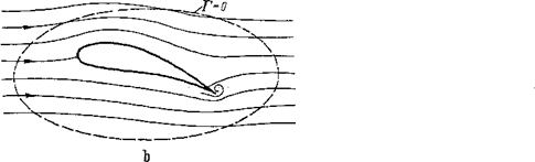
the conservation law of circulation in frictionless flow (Thomson theorem). This states that the circulation of a fluid-bound line is constant with time. This behavior will be demonstrated on a wing set in motion from rest, Fig. 2-7. Each fluid-bound line enclosing the wing at rest (Fig. 2-7a) has a circulation Г = 0 and retains, therefore, Г-0 at all later times. Immediately after the beginning of motion, frictionless flow without circulation is established on the wing (as shown in Fig.
2- 6a), which passes the sharp trailing edge from below (Fig. 2-lb). Now, because of friction, a left-turning vortex is formed with a certain circulation —Г. This vortex quickly drifts away from the wing and represents the so-called starting or initial vortex — Г (Fig. 2-lc).
For the originally observed fluid-bound line, the circulation remains zero, even though the line may become longer with the subsequent fluid motion. It continues, however, to encircle the wing and starting vortex. Since the total circulation of this fluid-bound line remains zero for all times according to the Thomson theorem, somewhere within this fluid-bound line a circulation must exist equal in magnitude to the circulation of the starting vortex but of reversed sign. This is the circulation +Г of the wing. The starting vortex remains at the starting location of the wing and is, therefore, some time after the beginning of the motion sufficiently far away from the wing to be of negligible influence on the further development of the flow field. The circulation established around the wing, which produces the lift, can be
replaced by one or several vortices within the wing of total circulation +Г as far as the influence on the ambient flow field is concerned. They are called the bound vortices.* From the above discussions it is seen that the viscosity of the fluid, after all, causes the formation of circulation and, therefore, the establishment of lift. In an inviscid fluid, the original flow without circulation and, therefore, with flow around the trailing edge, would continue indefinitely. No starting vortex would form and, consequently, there would be no circulation about the wing and no lift.
Viscosity of the fluid must therefore be taken into consideration temporarily to explain the evolution of lift, that is, the formation of the starting vortex. After establishment of the starting vortex and the circulation about the wing, the calculation of lift can be done from the laws of frictionless flow using the Kutta-Joukowsky equation and observing the Kutta condition.
 |
*In three-dimensional wing theory (Chaps. 3 and 4) so-called free vortices are introduced. These vortices form the connection, required by the Helmholtz vortex theorem, between the bound vortices of finite length that stay with the wing and the starting vortex that drifts off with the flow. In the case of an airfoil of infinite span, which has been discussed so far, the free vortices are too far apart to play a role for the flow conditions at a cross section of a two-dimensional wing. Therefore only the bound vortices need to be considered.
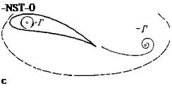 Figure 2-7 Development of circulation during setting in motion of a wing, (a) Wing in stagnant fluid. (b) Wing shortly after beginning of motion; for the liquid line chosen in {a), the circulation Г — 0; because of flow around the trailing edge, a vortex forms at this station, (c) This vortex formed by flow around the trailing edge is the so-called starting vortex — Г; a circulation +Г develops consequently around the wing.
2- 2-1 Kutta-J oukowsky Lift Theorem
Treatment of the theory of lift of a body in a fluid flow is considerably less difficult than that of drag because the theory of drag requires incorporation of the viscosity of the fluid. The lift, however, can be obtained in very good approximation from the theory of in viscid flow. The following discussions may be based, therefore, on inviscid, incompressible flow.[5] For treatment of the problem of plane (two-dimensional) flow about an airfoil, it is assumed that the lift-producing body is a very long cylinder (theoretically of infinite length) that lies normal to the
flow direction. Then, all flow processes are equal in every cross section normal to the generatrix of the cylinder; that is, flow about an airfoil of infinite length is two-dimensional. The theory for the calculation of the lift of such an airfoil of infinite span is also termed profile theory (Chap. 2). Particular flow processes that have a marked effect on both lift and drag take place at the wing tips of finite-span wings. These processes are described by the theory of the wing of finite span (Chaps. 3 and 4).
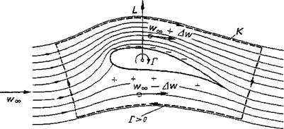
Lift production on an airfoil is closely related to the circulation of its velocity near-field. Let us explain this interrelationship qualitatively. The flow about an airfoil profile with lift is shown in Fig. 24. The lift L is the resultant of the pressure forces on the lower and upper surfaces of the contour. Relative to the pressure at large distance from tire profile, there is higher pressure on the lower surface, lower pressure on the upper surface. It follows, then, from the Bernoulli equation, that the velocities on the lower and upper surfaces are lower or higher, respectively, than the velocity w» of the incident flow. With these facts in mind, it is easily seen from Fig. 24 that the circulation, taken as the line integral of the velocity along the closed curve К, differs from zero. But also for a curve lying very close to the profile, the circulation is unequal to zero if lift is produced. The velocity field ambient to the profile can be thought to have been produced by a clockwise-turning vortex Г that is located in the airfoil. This vortex, which apparently is of basic importance for the creation of lift, is called the bound vortex of the wing.
In plane flow, the quantitative interrelation of lift L, incident flow velocity vv«,, and circulation Г is given by the Kutta-Joukowsky equation. Its simplified derivation, which will now be given, is not quite correct but has the virtue of being particularly plain. Let us cut out of the infinitely long airfoil a section of width b (Fig. 2-5), and of this a strip of depth dx parallel to the leading edge. This strip of planform area dA=bdx is subject to a lift dL = (рг—ри) dA because of the pressure difference between the lower and upper surfaces of the airfoil. The vector dL can be assumed to be normal to the direction of incident flow if the small angles are neglected that are formed between the surface elements and the incident flow direction.
The pressure difference between the lower and upper surfaces of the airfoil can be expressed through the velocities on the lower and upper surfaces by applying the
|
Figure 2-4 Flow around an airfoil profile with lift Z,. r = circulation of the airfoil. |
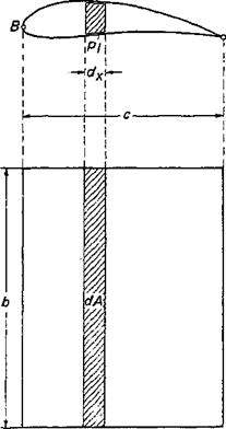 Figure 2-5 Notations for the computation of lift from the pressure distribution on the airfoil.
Bernoulli equation. From Fig. 2-4, the velocities on the upper and lower surfaces of the airfoil are (wM+ilw) and (w„ — dw), respectively. The Bernoulli equation then furnishes for the pressure difference
‘Ap=-pt — pu = (u’oo + A w)2 —|- (?./;oo — A w)2 = 2o v’oo A w
where the assumption has been made that the magnitudes of the circulatory velocities on the lower and upper surfaces are equal, Awi — Awu = Aw.
By integration, the total lift of the airfoil is consequently obtained as
|
Jap dA=b f dp dx (А) І |
(2-13 a) |
|
C 2gbWoo / Aw dx |
(2-13 b) |
|
J в |
The integration has been carried from the leading to the trailing edge (length of airfoil chord c).
The circulation along any line Taround the wing surface is
![]()
./’= Jwdl
(0
С В c
Г— fAwdx— f Aw dx — 2 f Aw dx (2-14 b)
B, u C, l В
The first integral in the first equation is to be taken along the upper surface, the second along the lower surface of the wing. From Eq. (2-13b) the lift is then given by
L = gbw00r (2-15)
This equation was found first by Kutta [35] in 1902 and independently by Joukowsky [31] in 1906 and is the exact relation, as can be shown, between lift and circulation. Furthermore, it can be shown that the lift acts normal to the direction of the incident flow.
2- 1 INTRODUCTION
In this chapter the airfoil of infinite span in incompressible flow will be discussed. The wing of finite span in incompressible flow will be the subject of Chap. 3, and the wing in compressible flow that of Chap. 4. More recent results and understanding of the aerodynamics of the wing profile are communicated in progress reports by, among others, Goldstein [19], Schlichting [56], and Hummel [26].
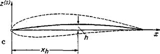
Wing profile The wing profile is understood to be the cross section of the wing perpendicular to the у axis. Accordingly, the profile lies in the xz plane and depends, in the general case, on the spanwise coordinate y. The geometry of a wing profile may be described, as in Fig. 2-1 a, by introducing the connecting line of the centers of the inscribed circles as the mean camber (or skeleton) line, and the line connecting the leading and trailing edges of the mean camber line as the chord. The greatest distance, measured along the chord, is called the wing or profile chord c. The largest diameter of the inscribed circles is designated as the profile thickness t (Fig. 2-1 b), and the greatest height of the mean camber line above the chord as the maximum camber h (Fig. 2-lc). The positions of the maximum thickness and the maximum camber are given by the distances xt (thickness position) and xh (camber position). The radius of the circle inscribed at the profile leading edge is taken as the nose radius rN it is usually related to the thickness. The trailing edge angle 2t
 |
Figure 2-1 Geometric terminology of lifting wing profiles, (a) Total profile, (jb) Profile teardrop (thickness distribution). (c) Mean camber (skeleton) line (camber height distribution).
(Fig. 2-16) is another important quantity. From these designated quantities the following six geometric profile parameters may be formed:
tjc relative thickness (thickness ratio)
h/c relative camber (camber ratio)[4]
xtjc relative thickness position
xhjc relative camber position
rNjc relative nose radius
2t trailing edge angle
For the complete description of a profile, the profile coordinates of the upper and lower surfaces, zu{x) and Z/(x), must also be known. A profile can be considered as originating from a mean camber line z^(x) on which is superimposed a thickness distribution (profile teardrop shape) z^x) > 0. For moderate thickness and moderate camber profiles, there results
zu, i(x) = z(sx) ± z(f)(x) (2-1)
The upper sign corresponds to the upper surface of the profile, and the lower sign to the lower surface.
For the following considerations, the dimensionless coordinates
X=- and Z = — (2-2)
c c
are introduced. The origin of coordinates, л: = 0, is thus found at the profile leading edge.
Of the large number of profiles heretofore developed, it is possible to discuss only a small selection in what follows. Further information is given by Riegels [50].
The first systematic investigation of profiles was undertaken at the Aerodynamic Research Institute of Gottingen from 1923 to 1927 on some 40 Joukowsky profiles [47]. The Joukowsky profiles are a two-parameter family of profiles that are designated by the thickness ratio t[c and the camber ratio h[c (see Sec. 2-2-3). The skeleton line is a circular arc and the trailing edge angle is zero (the profiles accordingly have a very sharp trailing edge).
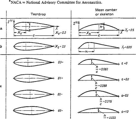
The most significant and extensive profile systems were developed, beginning in 1933, at the NACA Research Laboratories in the United States.* Over the years the original NACA system was further developed [1].
For the description of the four-digit NACA profiles (see Fig. 2-2a), a new parameter, the maximum camber position xh/c was introduced in addition to the thickness t/c and the camber hfc. The maximum thickness position is the same for all
|
c Figure 2-2 Geometry of the most important NACA profiles, (a) Four-digit profiles. (b) Five-digit profiles, (c) 6-series profiles. |
28 AERODYNAMICS OF THE WING profiles xtfc = 0.30. With the exception of the mean camber (skeleton) line for Xh = xh/c — 0.5, all skeleton lines undergo a curvature discontinuity at the location of maximum camber height. The mean camber line is represented by two connected parabolic arcs joined without a break at the position of the maximum camber.
For the five-digit NACA profiles (see Fig. 2-2b), the profile teardrop shape is equal to that of the four-digit NACA profiles. The relative camber position, however, is considerably smaller. A distinction is made between mean camber lines with and without inflection points. The mean camber lines without inflection points are composed of a parabola of the third degree in the forward section and a straight line in the rear section, connected at the station X—m without a curvature discontinuity.
In the NACA 6-profiles (see Fig. 2-2c), the profile teardrop shapes and the mean camber lines have been developed from purely aerodynamic considerations. The velocity distributions on the upper and lower surfaces were given in advance with a wide variation of the position of the velocity maximums. The maximum thickness position xtjc lies between 0.35 and 0.45. The standard mean camber line is calculated to possess a constant velocity distribution at both the upper and lower surfaces. Its shape is given by
g(s) = — — in 2[(1 — AT) In (1 —X) + ХЫ X] (2-3)
c
A particularly simple analytical expression for a profile thickness distribution, or a skeleton line, is given by the parabola Z = aX( 1 ~X). Specifically, the expressions for the parabolic biconvex profile and the parabolic mean camber line are
Z^X) = 2 — X(l — X) (24 a)
Z<-s)=4^X(l – X) (24b)
Here, t is the maximum thickness and h is the maximum camber height located at station X = .
The so-called extended parabolic profile is obtained by multiplication of the above equation with (1 + bX) in the numerator or denominator. According to
,Glauert [17], such a skeleton line has the form
/ I * *
‘.У: ?’Г/ ‘—————– -3 = aX( – m + ЬХ) (2-5)
Usually these are profiles with inflection points.
According to Truckenbrodt [49], the geometry of both the profile teardrop shape and the mean camber line can be given by
– ■■ X(l — X)
У……………. ^ Z{X) = a (2-6)
For the various values of b, this formula produces profiles without inflection points that have various values of the maximum thickness position and maximum camber position, respectively. The constants a and b are determined as follows:
|
Teardrop: |
1 t a 2Xf c |
l-2Xt b~ X2 |
(2-7 a) |
|
Skeleton: |
1 h a X2hc |
, 1 – 2Xa 4= XI |
(2-74) |
Of the profiles discussed above, the drop-shaped ones shown in Fig. 2-2 have a rounded nose, whereas those given mathematically by Eq. (2-6) in connection with Eq. (2-7a) have a pointed nose. The former profiles are therefore suited mainly for the subsonic speed range, and the latter profiles for the supersonic range.
Pressure distribution In addition to the total forces and moments, the distribution of local forces on the surface of the wing is frequently needed. As an example, in Fig. 2-3 the pressure distribution over the chord of an airfoil of infinite span is presented for various angles of attack. Shown is the dimensionless pressure coefficient
 |
|
|
|
![Подпись: with the profile NACA 2412 [12]. Reynolds number Re = 2.7 • IQ6. Mach number Ma = 0.15. Normal force coefficients according to the following table:](/img/3131/image059_2.png)
versus the dimensionless abscissa x/c. Here ip — Poo) is the positive or negative pressure difference to the pressure p„ of the undisturbed flow and, the dynamic pressure of the incident flow. At an angle of attack a = 17.9°, the flow is separated
|
cc |
-1.1° |
2.8° |
7.4° |
13.9° |
17.8° |
|
-CZ |
0.024 |
0.433 |
0.862 |
1.356 |
0.950 |
from the profile upper surface as indicated by the constant pressure over a wide range of the profile chord.
 |
 |
The pressures on the upper and lower surfaces of the profile are designated as pu and pi, respectively (see Fig. 2-3), and the difference Ар = (рг — pu) is a measure for the normal force dZ= A pb dx acting on the surface element dA = b dx (see Fig. 2-5). By integration over the airfoil chord, the total normal force becomes
where cz is the normal force coefficient from Eq. (1-21) (see Fig. 2-3). For small angles of attack a, the negative value of the normal force coefficient can be set equal to the lift coefficient cL:
 (2-10)
The pitching moment about the profile leading edge is
M=—b / Ap{x)dx (2-lla)
X)
= cMqaobc’1 (2-11 b)
where nose-up moments are considered as positive. The pitching-moment coefficient is, accordingly,
![]()
![]()
 (2-12)
Motion modes of the airplane After having discussed the aerodynamic forces and the moments acting on the aircraft, its modes of motion may now be described briefly. An airplane has six degrees of freedom, namely, three components of translational velocity Vx, Vy, Vz, and three components of rotational velocity cox, coy, coz. They can be expressed, for instance, relative to the aircraft-fixed system of axes x, y, z as in Fig. 1-6. The components of the aerodynamic forces, as introduced in Sec. 1-3-2, and their dimensionless aerodynamic coefficients are functions of these six degrees of freedom of motion.
The steady motion of an aircraft can be split up into a longitudinal and a lateral motion. During longitudinal motion, the position of the aircraft plane of symmetry remains unchanged. It is characterized by the three components of motion
Vx, Vz, со у (longitudinal motion)
The remaining three components determine the lateral motion
Vy, ojx, coz (lateral motion)
It is expedient for the analysis of the interrelation of aerodynamic coefficients and components of motion to break down the general motion into straight flight, as described by Vx and Vz yawed flight, described by Vy; and rotary motion about the three axes. These rotary motions are, specifically, the rolling motion cox, the pitching motion coy, and the yawing motion coz. The quantities of angle of attack a and angle of yaw j3,[3] which were introduced earlier (see Fig. 1-6), are then given by
V f V f
tan a = —- and tan (3 = (1-22)
*xf ^xf
The signs of a, jS, cox, ojy, and cj2 can be seen in Fig. 1-6. At unsteady states of flight, the aerodynamic forces also depend on the acceleration components of the motion.
Forces and moments during straight flight The incident flow direction of an airplane in steady straight flight is given by the angle of attack a (Fig. 1-6).’The resultant aerodynamic force is fixed in magnitude, direction, and line of application by lift L, drag D, and pitching moment M (Fig. 1-6). Let us now give some details on the dimensionless aerodynamic coefficients introduced in Sec. 1-3-2. For moderate angles of attack, the lift coefficient cL is a linear function of the angle of attack a:
cL = (a — a0 ) — (1-23)
where aQ is the zero-lift angle of attack and dcLjda is the lift slope. A further characteristic quantity for the lift is the maximum lift coefficient cLmax, which is reached at an angle of attack that depends on the airplane characteristics.
For moderate angles of attack and lift coefficients, the drag coefficient cD is given by
Cd = cdo +kiCL + k2c (1-24)
where cDо is the drag coefficient at zero lift (form drag). The constants kx and k2 depend mainly on the wing geometry.
For wings of symmetric profile without twist we have kx ~ 0, and thus
cd = cdo + k2c (1-25)
This is the representation of the drag polar.
The pitching-moment coefficient см is a linear function of the angle of attack a and the lift coefficient cL, respectively:
cm = cMo±^~-Cl 0-26)
where смо is the zero-moment coefficient and dcM/dci is the pitching-moment slope. The value of cM0 is independent of the choice of the moment reference
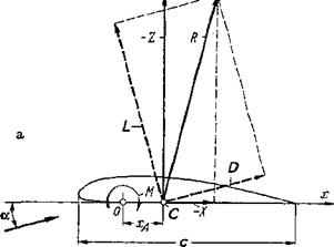
station, whereas dcMjdcL depends strongly on it. The quantity dcMjdcL is also called the “degree of stability of longitudinal motion” (rotation about lateral axis). The resultant of the aerodynamic forces of the airplane is completely determined only when its magnitude, direction, and the position of its line of application are known. These three data are obtained, for instance, from lift, drag, and pitching moment. The position of the line of application of the resultant R, for example, on the wing, can be defined as the intersection of the line of application with the profile chord (Fig. l-7a). This point is called the center of pressure or aerodynamic center of the wing. With xA, the distance of the center of pressure from the moment reference axis, we have
M=xAZ
For small angles of attack, the normal force with the negative sign is, in first approximation, equal to the lift:
Z=-L
and by introducing the nondimensional coefficients,
 xl __ cm
Cjx C%
 |
_ CM _ dcM Cm 0 cL dcL cL
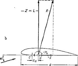 Figure 1-7 Demonstration of location of aerodynamic center (center of pressure). {a) Aerodynamic center C. (b) Neutral point N. In general, the reference wing chord is с = Сд.
This relationship means that the position of the center of pressure generally varies with the lift coefficient. The shift of the center-of-pressure position is given by the term —cmo/cl-
In agreement of theory with experiment, the pitching moment can generally be described as the sum of a force couple independent of lift (zero moment) and a term proportional to the lift:
M = M0 ~xnL
In words, the pitching moment is the sum of the zero moment and of the moment formed by the lift force and the distance xN between the neutral point and the moment reference line (Fig. 1-7Й). Again introducing the non – dimensional coefficients for lift and pitching moment:
![]()
![]() _ ■ XN
_ ■ XN
cm – cmo _ CL
CjU
Comparison with Eq. (1-26) yields, for the position of the neutral point
^N_ _ dcM CH dcL
which shows that the pitching-moment slope dCj^ldcL determines the position of the neutral point. The terms dcLjda and dc^lda. are designated as derivatives ■of longitudinal motion.
Forces and moments in yawed flight When an aircraft is in stationary yawed flight, the direction of the incident flow of the wing is determined by both the angle of attack a and the angle of sideslip 0 (Fig. 1-6). Because of the asymmetric flow incidence, additional forces and moments are produced besides lift, drag, and pitching moment as discussed in the last section. The force in direction of the lateral axis у is the side force due to sideslip; the moment about the longitudinal axis, the rolling moment due to sideslip; and the moment about the vertical axis, the yawing moment due to sideslip. The derivatives for /3=0,
/9с y / дсмЛ / ЭсмД
‘ 90/0= о 90 /0=о V 90 /0=о
are called stability coefficients of sideslip; in particular, 9c^z/90 is called directional stability. All three of these coefficients are strongly dependent on the wing sweepback, besides other influences.
Forces and moments in rotary motion An airplane in rotary motion about the axes x, y, z, as specified by the modes of motion of Sec. 1-3-3, is subject to additional velocity components that are produced, for example, locally on the wing and that change linearly with distance from the axis of rotation. The aerodynamic forces and moments that are the result of the angular velocities cox, сcy, coz will now be discussed briefly.
During rotary motion of the airplane about the longitudinal axis (roll) with
angular velocity ojx, the lift distribution on the wing, for instance, becomes antisymmetric along the wing span. The resulting moment about the x axis can be called a rolling moment due to roll rate. It always counteracts the rotary motion and is, therefore, also called roll damping. The asymmetric force distribution along the span produces also a yawing moment, the so-called yawing moment due to roll rate. Introducing the dimensionless coefficients according to Eq. (1-21), the stability coefficients of sideslip
are obtained.
The quantity Qx is the dimensionless angular velocity ojx. It is obtained from ojx, the half-span s, and the flight velocity V:
= (1-30)
The rotary motion of an airplane about the vertical axis (yaw) produces additional longitudinal air velocities on the wing that have reversed signs on the two wing halves and that result in an asymmetric normal and tangential force distribution along the wing span, which in turn produces a rolling and a yawing moment. The yawing moment created in this way counteracts the rotary motion and is called yawing or turning damping. The rolling moment is called rolling moment due to yaw rate. Again by introducing nondimensional coefficients after Eq. (1-21), further stability coefficients of yawing motion are formed:
^смх д°м2
and а<27
Here the nondimensional yawing angular velocity is
The rotary motion of the aircraft about the lateral axis (pitch), Fig. 1-6, produces on the wing an additional component of the incident velocity in the z direction that is linearly distributed over the wing chord. This results in an additional lift due to pitch rate and an additional pitching moment that counteracts the rotary motion about the lateral axis. Therefore, it is also called pitch damping of the wing. The magnitude of the pitch damping is strongly dependent on the position of the axis of rotation (y axis). By using lift and pitching-moment coefficients after Eq. (1-21), the following additional stability coefficients of longitudinal motion are obtained:
(1-32)
![]()
is made dimensionless with wing reference chord cM after Eq. (3-5b) contrary to the rolling and yawing angular velocities Qx and Qy, respectively, which were made dimensionless with reference to the wing half-span.
Only the most important aerodynamic forces and moments produced by the rotary motion of the aircraft have been discussed above. Omitted, for instance, were detailed discussions of the side forces due to roll rate and yaw rate.
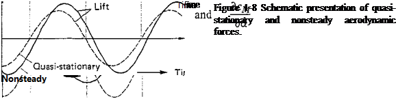
Forces and moments in nonsteady motion Besides the steady aerodynamic coefficients discussed above, the nonsteady coefficients applicable to accelerated flight have increasingly gained importance, particularly for flight mechanical stability considerations. Nonsteady motions are more or less sudden transitions from one steady state to another or time-periodic motions superimposed on a steady motion. If the periodic motion is very slow (e. g., changes of angle of attack), the aerodynamic forces can be computed from quasi-stationary theory; this means that, for instance, the momentary angle of attack determines the forces. With periodic motions of higher frequency, however, the aerodynamic forces are phase-shifted (leading or lagging) from the motion. These conditions are demonstrated schematically in Fig. 1-8 for an airplane undergoing a periodic translational motion normal to its flight path.
 |
At nonsteady longitudinal motion, new aerodynamic force coefficients must be used, for example, the derivatives
 |
where a = docjdt is the timewise change of the angle of attack. The nonsteady coefficients are important both for flight mechanics of the aircraft, assumed to be inflexible, and for questions concerning the elastically deformable airplane (aero- elasticity).
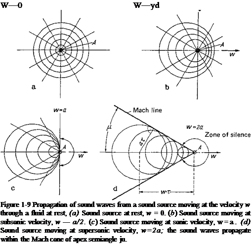
Forces and moments in supersonic flight During the transition from subsonic to supersonic flight, the aerodynamic behavior of an airplane undergoes a basic change. This becomes obvious when the airplane is taken as the source of a disturbance that moves through still air at a velocity V = w. Relative to this moving center of disturbance, pressure waves emanate with the speed of sound a. A closer investigation of this process shows the importance of the speed of sound—especially the ratio of flight velocity to sonic speed, that is, the Mach number from Eq. (1-16). In terms of fluid mechanics, the airplane can be considered as a sound source. Figure 1-9д shows the propagation of sound waves from a sound source at rest on concentric spherical surfaces. In Fig. 1-9b the sound waves, emitted at equal time intervals, can be seen for a source that moves with one-half the speed of sound, w = a[2. Figure l-9c is the corresponding picture for w = a and finally, Fig. 1-9d is for w — 2a. In this last case, in which the sound source moves at supersonic velocity, the effect of the source is felt only within a cone with the apex semiangle ju, which is given by
This cone is called the Mach cone. No signals can be sent from the source to points outside of the Mach cone, a zone called the zone of silence. No sound is heard, therefore, by an observer who is being approached by a body flying at supersonic speed. Physically, the process described is obviously identical to a sound source at rest in a fluid approaching from the right with velocity w. We have to keep in mind, therefore, the following characteristic difference: When the fluid velocity is smaller than the speed of sound (w<a, subsonic flow), pressure disturbances propagate in all directions of space (Fig. 1 -9b). When the fluid velocity is greater than the speed of sound, however (w>a, supersonic flow), pressure disturbances can propagate only within the Mach cone situated downstream of the sound source (Fig. 1-9(2).
Now, every point of the airplane surface can be considered as the source of a disturbance (sound source) as in Fig. 1-9, in analogy to the previous discussion where the whole airplane was taken as the sound source. It can be concluded, therefore, that because of the different kinds of propagation of the individual pressure disturbances as in Fig. 1 -9b and d, the pressure distribution and consequently the forces and moments on the various parts of the airplane (wing, fuselage, control surfaces) depend decisively on the airplane Mach number, whether the airplane flies at subsonic or supersonic velocities.
The above considerations show that subsonic flow has the characteristic properties of incompressible flow, whereas supersonic flow is basically different. In most cases, therefore, it will be expedient to treat subsonic and supersonic flows separately.
REFERENCES
1. Lilienthal, O.: “Der Vogelflug als Grundlage der Fliegekunst,” 1889; 4th ed., Sandig, Wiesbaden, 1965.
2. “U. S. Standard Atmosphere,” National Oceanic and Atmospheric Administration and National Aeronautics and Space Administration, Washington, D. C., 1962.
Lift, drag, and lift-drag ratio Airplanes moving with constant velocity are subject to an aerodynamic force R (Fig. 1-5). The component of this force in direction of the incident flow is the drag D, the component normal to it the lift L.
Lift is produced almost exclusively by the wing, drag by all parts of the aircraft (wing, fuselage, empennage). Drag will be discussed in detail in the following chapters. It has several fluid mechanical causes: By friction (viscosity, turbulence) on the surfaces, friction drag is produced, which is composed of shear-stress drag and a friction-effected pressure drag. This kind of drag depends essentially on the aircraft geometry and determines mainly the drag at zero lift. It is called form drag or also profile drag. As a result of the generation of lift on the wing, a so-called induced drag is created in addition (eddy drag), which depends strongly on the aspect ratio (wing span/mean wing chord). An aircraft flying at supersonic velocity is subject to a so-called wave drag, in addition to the kinds of drag mentioned above. Wave drag is composed of a component for zero lift (form wave drag) and a component caused by the lift (lift-induced wave drag).
The inclination of the resultant R to the incident flow direction and consequently the ratio of lift to drag depend mainly on wing geometry and incident flow direction. A large value of this ratio L/D is desirable, because it can be considered to be an aerodynamic efficiency factor of the airplane. This efficiency factor has a distinct meaning in unpowered flight (glider flight) as can be seen from Fig. 1-5. For the straight, steady, gliding flight of an unpowered aircraft, the resultant R of the aerodynamic forces must be equal in magnitude to the weight W but with the sign reversed. The lift-drag ratio is given, therefore, after Fig. 1-5, by the relationship
where є is the angle between flight path and horizontal line.
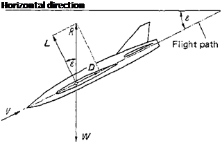 Figure 1-5 Demonstration of glide angle z.
The minimum glide angle is a very important quantity of flight
performance, particularly for glider planes. It is given by (I//Z))max after Eq. (1-18). The outstanding characteristic of the wing, in comparison to the other parts of the aircraft, is its quite large lift-drag ratio. Here are a few data on L/D for incompressible flow: A rectangular plate of an aspect ratio A = b/c = 6 has a value of (L/D)max of
6- 8. Considerably greater lifts for about the same drag are obtained when the plate is somewhat arched. In this case (L/D)max reaches 10-12. Even more favorable values of (L/D)max are obtained with wings that are streamlined. Particularly, the leading edge should be well rounded, whereas the profile should taper out into a sharp trailing edge. Such a wing may have an (L/D)max of 25 and higher.
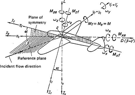
Further forces and moments, systems of axes We saw that, for symmetric incident flow, the resultant of aerodynamic forces is composed of lift and drag only. In the general case of asymmetric flow, the resultant of the aerodynamic forces may be composed of three forces and three moments. These six components correspond to six degrees of freedom of the aircraft motion. We introduce two systems of axes, depending on the flight mechanical requirements, to describe these forces and moments (Fig. 1-6).
1. Airplane-fixed system: Xf, y/, Zf
2. Experimental system: xe, ye, ze
The origin of the coordinates is the same in the two systems and is located in the symmetry plane of the aircraft. Its location in this plane is chosen to suit the specific problem. For flight mechanical studies, the origin is usually put into the aircraft center of gravity. For aerodynamic computations, however, it is preferable to put the origin at a point marked by the aircraft geometry. In wing aerodynamics it is advantageous to choose the geometric neutral point of the aircraft, as defined in Sec. 3-1.
The lateral axes of the experimental system of axes xe, ye, ze and of the system fixed in the airplane Xf, yf, Zf coincide so that ye = У/. The experimental system is obtained from the airplane-fixed system by rotation about the lateral axis by the angle a (angle of attack) (Fig. 1-6). .
For symmetric incident flow, the aerodynamic state of the aircraft is defined by the angle of attack a and the magnitude of the velocity vector. For asymmetric incidence, the angle of sideslip /3[2] is also needed. It is defined as the angle between the direction of the incident flow and the symmetry plane of the aircraft (Fig.
1- 6).
|
Figure 1-6 Systems of flight mechanical axes: airplane-fixed system, Xp yp zp experimental system, xe, ye, ze; angle of attack, a; sideslip angle, jS; angular velocities, cox, wy, ojz. |
Forces and moments in the two coordinate systems are defined as follows:
1. Aircraft-fixed system:
Xf axis: tangential force Xf, rolling moment MXf У/ axis: lateral force Yp pitching mdment Mf (or My/) ip axis: normal force Zp yawing moment MZf
2. Experimental system:
xe axis: tangential force Xe, rolling moment Mxe уe axis: lateral force Ye, pitching moment Me (or Mye) ze axis: normal force Ze, yawing moment Mze
The signs of forces and moments are shown in Fig, 1-6.
It is customary to use lift L and drag D in addition to the forces and moments. They are interrelated as follows:
L = – Ze D = – Xe (for (3 = 0) (1-19)
Further, because of the coincidence of the lateral axes y/ = ye,
Yf= Ye Mf = Me =M (1-20)
Dimensionless coefficients of forces and moments For the representation of experimental results and also for theoretical calculations, it is expedient to introduce dimensionless coefficients for the moments and forces defined in the preceding paragraph. These coefficients are called aerodynamic coefficients of the aircraft. They are related to the wing area Aw, the semispan 5, the reference wing chord cM (Eq. 3-5b), and to the dynamic pressure q ~ pV2 J2, where V is the flight velocity (velocity of incident flow). Specifically, they are defined as follows.
|
Lift: |
L = clA ц/q |
|
Drag: |
D = cD A wq |
|
Tangential force: |
X= cxAwq |
|
Lateral force: |
Y=cyAwq |
|
Normal force: |
Z = czA wq |
|
Rolling moment: |
■— ці sq |
|
Pitching moment: |
M = СмАц/c^q |
|
Yawing moment: |
Mz = cMzAwsq |
A measurement that determines the three coefficients cL, cD, and cM as a function of the angle of attack a is called a three-component measurement. The diagram cL(cD) with a as the parameter was introduced by Lilienthal [1]. It is called the polar curve or the drag polar. If all six components are measured, for example, of a yawed airplane, such a test is called a six-component measurement. Normally, the coefficients of forces and moments of aircraft depend considerably on the Reynolds number Re and the Mach number Ma in addition to the geometric data. At low flight velocities, however, the influence of the Mach number on force and moment coefficients is negligible.