Category Dynamics of. Atmospheric Flight

TRANSFER FUNCTIONS

TRANSFER FUNCTIONS Подпись: (3.2,1)

System analysis frequently reduces to the calculation of system outputs for given inputs. A convenient and powerful tool in such analysis is the transfer function, a function G(s) of the Laplace transform variable s that relates a particular input x(t) and output y(t) as follows,

where (_) denotes the Laplace transform (see See. 2.3). So long as x(t) and y(t) are Laplace transformable the transfer function defined by (3.2,1) exists. However, it will in general be a function of the initial values of у and its derivatives, and moreover, for nonlinear and time-varying systems, of the particular input x(t) as well. Such a transfer function is of relatively little use. We can however obtain a unique function G(s) if (i) the system is linear and time invariant, and (ii) it is initially quiescent, i. e. at rest at the origin in state space with no inputs. We shall therefore restrict ourselves in the following to this special situation. (A companion concept, the describing function, useful for nonlinear systems is described in Sec. 3.5.) With a unique transfer function, the output y(t) for any input x(t) is found by taking the inverse Laplace transform of

y(s) = ЩаЩа) (3.2,2)

The transfer function is thus seen to be the mathematical embodiment of all the system characteristics relevant to the particular input/output pair. For linear/invariant systems, we shall see below that the computation of G(s) is always possible in principle, and usually in practice.

When, as required above, x(t) and y(t) are zero for t < 0, the Laplace and Fourier transforms are simply related, i. e. x(ico) = X((o). It follows that

G(ia>) = (3.2,2a)

X(a>)

Sometimes it is G(ia>) that is called the transfer function.

With a multivariable system, there is more than one input/output pair. In that case, let G^s) be the transfer function that relates the output y((t) to the input x5(t). All the input/output relations are then given by

m

¥i(s) = 2 Ga(8) Vj(s) (3.2,3a)

3-1

or

У («) = вї(«) (3.2,36)

where

G = [<?„(«)] (3.2,3c)

is an n X m matrix associated with n outputs and m inputs. It need not be square since one output can be influenced by any number of inputs and vice versa. Note from (3.2,3a) that

TRANSFER FUNCTIONS

STATIC GAIN

Consider the output y(t) that results from the unit-step input x(t) = 1 (t). From Table 2.3, item 3, the transform of the input is


*(«) = –

s


and hence


. G(s)

y{s) = —

s


The final value theorem (2.3,17) therefore gives

lim y(t) = lim sy(s) = lim G(s)

і-►oo s->0 s-*0

This limit is the static gain, K, so that

К = lim G(s)

s-»0


(3.2,4)


EXAMPLE


TRANSFER FUNCTIONS

(3.2,5)


f(s) s2 + 2^o)ns + m2 The static gain К is found to be


К = lim G(s) = – L


(3.2,6)


SYSTEMS IN SERIES

When two subsystems are in series, as in Fig. 3.4, the overall transfer function is

G(s) = £(£) = !i£). Sif) ж(а) y(s) x(s)


whence


G(s) = 6,(3) ■ G2(s)


TRANSFER FUNCTIONS

x


У


z


Gi(s)


G2(s)


Fig. 3.4 Systems in series.


Similarly, for n subsystems in series, the result is

в(8) = <?,(«) ■ G2(s) ■ • • 0n(s)


(3.2,7)


SYSTEM WITH FEEDBACK

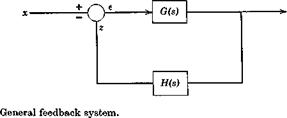
Figure 3.5 shows a general feedback arrangement, containing two sub­systems. When used as a feedback controller, € is called the actuating signal, f G(s) the forward-path transfer function and H(s) the feedback transfer function. As indicated e is the difference between x and z, so


e = x — z у = G(x — z) z = Hy


whence it follows easily that the overall transfer function is


У G x 1 + GH


(3.2,8)


and the actuating-signal transfer function is


I – 1

x 1 + GH


(3.2,9)


Fig. 3.5


t The designation error is reserved for the difference x — y, the aim of such a control system being to force у to be equal to x.


TRANSFER FUNCTIONS

TRANSFER FUNCTIONS

EQUILIBRIUM, CONTROL, AND STABILITY

Equilibrium denotes a steady state of the system, one in which all the state variables are constant in time. The “motion” corresponding to equilib­rium is represented by a point in the state space. The nonautonomous inputs associated with equilibrium must be zero or constant, the zero case preferably corresponding to the equilibrium point at the origin. The usual way of changing the equilibrium state, i. e. of exercising control over the system is by means of the nonautonomous inputs, the appropriate subset of which can hence be termed the control vector, and the associated space the control space. The result of applying control is to cause the equilibrium point to move away from the origin in state space, and the locus of all its possible positions defines a region that is a map of the domain of the control vector in control space. The control is adequate only if this region contains all the desired operating states of the system (e. g. orientation angles and speeds of a flight vehicle).

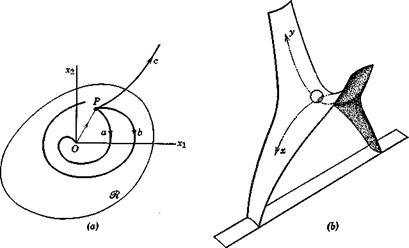
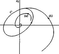
Stability embraces a class of concepts that, while readily appreciated intuitively, are not easily defined in a universal way. In the past, a common view of system stability has been that it is a property of the equilibrium state, as follows. Let a system be in equilibrium, and for convenience let the equilibrium point be chosen as the origin of state space. Now let the initial state for the autonomous system be at a point P (see Fig. 3.3a) in the immediate neighborhood of 0. Three possibilities exist for the subsequent motion, illustrated by the three trajectories a, b, and c in the figure.

(а) The state point moves back to the origin.

(б) It remains finite but >0 for all subsequent time

(c) It goes off to infinity.

The trajectory will of course, for a given system, depend on the direction of OP in state space. For example, Fig. 3.36 shows the equilibrium of a ball on a saddle surface. It is evident that displacement in the x direction leads to a type (c) trajectory and displacement in the у direction (in the presence of damping) to one of type (a). In this view of stability, the equilibrium point would be said to be stable if only type (a) trajectories could occur regardless of the direction of OP, and unstable if type (c) trajectories could occur. The saddle point is therefore an unstable equilibrium. The question of the magnitude of OP must be considered as well. If the system is linear, the conclusion about stability is independent of the magnitude of OP, but if it is not the size of the initial disturbance (i. e. of OP) does matter. It may well be that the system is stable for small disturbances, but unstable for large ones, as illustrated in Fig. 3.3c. The initial states for which the origin is stable in such a case lie within some region 0t of the state space as illustrated in Fig. 3.3a, and this is the “region of stability of 0.”

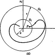
More recently, the rediscovery of the work on stability by Lyapunov (ref. 3.2) (see also Sec. 3.5) has had a great influence on this subject. In the Lyapunov viewpoint, we speak not of the stability of a system, but of the stability of a particular solution of a system of equations. The solution may be quite general, for example the forced motion of a nonlinear time-varying system with particular initial conditions. Equilibrium is a special case of such a solution. In this special case the Lyapunov definition is as follows. Let <5 and e be the radii of two hyperspheres in state space with centers at the equilibrium point, symbolically represented in two dimensions in Fig. 3.3d. These surfaces are such that for all initial states lying inside Sx the subsequent solution lies for all time inside S2. Then the origin is a stable point if there exists a д > 0 for all e > 0, no matter how small є becomes. That is, the solution can be made arbitrarily small by choosing the initial conditions small enough. If the solutions tends ultimately to zero, then the origin is asymptotically stable. If, when 0 is asymptotically stable, there exists a region M such that all trajectories that originate within it decay to the origin, then ЗІ is a finite region of stability. This notion is identical with that previously described. If 01 is an infinite sphere then the origin is globally stable. Note that if a linear system is asymptotically stable it is also globally stable. This fact is somewhat academic since in nature “linear” systems always become nonlinear for “very large” state vectors.

The Lyapunov condition for a region of stability ЗІ will be met whenever the solution is a “well-behaved” function of the initial conditions—that is, if Эжг(Т)/Эж3(0) is finite in ЗІ for all i, j and T where x is the state vector. In particular this must hold in the limit as T —* oo.

A striking illustration of this point of view is afforded by the unstable

EQUILIBRIUM, CONTROL, AND STABILITY

(с)


EQUILIBRIUM, CONTROL, AND STABILITY

EQUILIBRIUM, CONTROL, AND STABILITY

EQUILIBRIUM, CONTROL, AND STABILITY

(f)

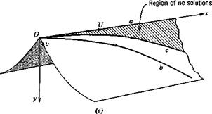
Fig. 3.3 Stability of equilibrium, (a) Trajectories in state space. (6) Saddle point, (c) Finite region of stability. (d) Lyapunov definition of stability, (e) Illustrating discontinuity in solutions. (/) Limit cycle.

system of Fig. 3.3e, in which a particle is free to slide without friction along a horizontal pointed ridge. The sides are infinite in the x and у directions. One solution, of course, is uniform rectilinear motion at speed U on the ridge (trajectory a). If a small initial tangential velocity v in the downhill direction be added, the motion is a trajectory such as b. In the limit as v —»■ 0, the limiting trajectory is one like c, tangent to Ox at the origin. Thus there is a gap between a and c that contains no solutions at all for the given U even for finite times. If the top of the ridge were rounded off instead of pointed the solutions for all finite t would be continuous in v. However even in that case, as t -> oo the lim yfv —*■ oo, so that 2/(00) is not a continuous

. v—>-0

function of v, and hence the basic solution a is unstable.

When the solution to be investigated is not the simple one discussed above, i. e. equilibrium, the stability criterion is still that of continuity, as above.

Alternatively, the general case can be reduced to the particular case as follows. Let the system equation be

x = f(x, t) (3.1,1)

and let the particular solution be x0(f). Now let the variation from x0 asso­ciated with a change in the initial condition only be

у = X(t) — x0(t) (3.1,2)

Подпись:У = x(0 — xoW

= f(x> t) – f(x0. t)

Подпись: orУ = % + xo(<)> t) – f(xo(0> t) (3-1.3)

Since x0(f) is presumed known, then (3.1,3) is an equation of the form

У = g(y, *) (3-1,4)

for which у = 0 is the solution corresponding to x(f) = x0(f). Thus (3.1,4) defines a system that has an equilibrium point at the origin, and the discussion of its stability has already been given. In this way the stability of any tran­sient solution is reduced to that of stability of equilibrium.

A particular kind of solution that is of interest is the limit cycle, illustrated again in two dimensions, in Pig. 3.3/ by the closed curve G. It may be orbitally stable, in which case neighboring trajectories such as (6) are asymptotic to it, or unstable, in which case neighboring trajectories such as (a) starting arbitrarily close to C, never come back to it.

Finally, we should remark that Lyapunov’s definition is concerned only with variations in the initial conditions of a solution. Clearly there are two other important practical cases: (1) stability with respect to perturbations in the input, and (2) stability with respect to system or environmental parameters. Stability with respect to perturbations in the input or the system parameters can be defined in a manner quite analogous to that with respect to the initial conditions.

LINEARITY AND TIME INVARIANCE

A system is linear if its governing equations are linear in the state variables. In that case the time functions giving the state variables are simply pro­portional to the magnitude of nonautonomous input functions of given shape when the initial conditions are zero, and to the initial conditions if there are no nonautonomous inputs. If the parameters of the system and of the environment are constants, then the system is time invariant. The simplest class of systems is that which has both these properties—linearity and time invariance—and these can be completely analyzed by the available methods of linear mathematics. We shall denote these as linearjinvariant systems. Departure from either of these conditions leads to mathematical problems for which there may be no general methods of solution apart from numerical computation.

BLOCK DIAGRAM

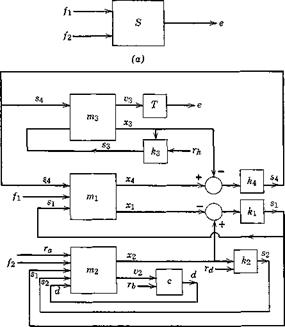
The input/output system relations are conveniently illustrated by the use of block diagrams, as in Fig. 3.2. Figure 3.2a is the overall system diagram showing inputs f1 and /2 and output e and Fig. 3.26 is the combined block diagram of the subsystems, showing the sort of interconnections and feed­backs that are typically encountered in real systems.

BLOCK DIAGRAM

(b)

Fig. 3.2 Block diagram, (a) Complete system. (6) Detailed block diagram. = spring forces, d = damper force. ri = reaction forces.

EXAMPLE

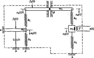
Figure 3.1 shows a system S comprising a planar arrangement of rigid bodies mit massless springs Jct, viscous damper c, and an inductive displace­ment transducer T. (Its voltage is e(t) = const. x3.) The midpoint g of т1г and mass m3, are constrained to move vertically. The system, bounded by the dashed line, is made up of all these separate elements. The nonautonomous

EXAMPLE

Fig. 3.1 An example of a system.

inputs are the arbitrary external forces and /2 acting on the masses and the state variables are the coordinates of the joints, xft), their velocities vft) = xit and the voltage e{t) of the transducer. Any of this set might be taken as outputs. Here, however, the output happens to be e(t). If fx and/2 were zero, the system would be autonomous and capable only of free vibration associated with nonequilibrium initial conditions. The external reactions at the points of connection to the fixed base, a, b, d, h, and g are functions of the state variables xi and vit and hence are autonomous inputs. The parameters of the system are the masses of mt, the stiffnesses of Jcit the damping constant of c, the transducer constant, and the geometrical di­mensions. It should be pointed out that although there is a minimum number of coordinates (state variables xt and vf) required to specify the state of the system, eight in this example, this number may be arbitrarily increased by redundant variables if it is convenient to do so. For example, we might add the transducer output, the four accelerations a( = vf, and the forces in the springs, even though they are, by virtue of the physical laws governing the system, not independent of the x( and vt. (Indeed the mathematical statement of this dependence is the main ingredient in the formulation of the system equations.) The minimum number of state variables required is the order of the system.

The arbitrariness of the choice of system, and its dependence on the aim of the investigation is illustrated by the fact that we might choose as a system for study any of the individual elements of S, or any of the subsystems obtained by combinations of them. Furthermore, the set of state variables might be still further augmented by adding sudh items as the stresses and strains in m1 and m2.

Finally, the release of simplifying approximations such as rigidity of the bodies, and masslessness of the springs, would require further elaborate additions to the state variables.

System Theory

CHAPTER 3

3.1 CONCEPTS AND TERMINOLOGY

The branch of modem engineering analysis known as system theory is highly relevant to the study of the flight of vehicles in the atmosphere and in space. The word system has long been current in such applications as “control system,” “navigation system,” and “hydraulic system.” In our present context we identify the vehicle itself as a system, of which the above examples are subsidiary systems, or associated systems.

We do not attempt to offer here a precise definitionf of a system—suffice it to say that it is an element, or an interconnected set of elements that is clearly identifiable and that has a state defined by the values of a set of vari­ables that characterize its instantaneous condition. The elements may be physical objects or devices, or they may be purely mathematical, i. e. equations expressing relationships among the variables. In the case of a physical system, the governing equations may or may not be known. A set of equations that constitutes a mathematical model of a physical system, is a mathematical system that is a more or less faithful image of the physical system, depending on the assumptions and approximation contained therein. The set of n variables that defines the state of the system is the state vector,

f See for example ref. 3.1, Sec. 1.10.

and the corresponding те-dimensional space is the state space. Some or all of the state variables, or quantities derived from them, are arbitrarily termed, according to the circumstances of the experiment or analysis, as outputs. The exact specification of a system is usually arbitrary, as will be seen in the following example; the “boundary” of the system under consideration in any given circumstance is chosen by the analyst or experimenter to suit his purpose.

In addition to the state variables, there is usually associated with a system a second set of variables called inputs. These are actions upon the system the physical origins of which are outside the system. Some of these are independent of the state of the system, being determined by processes entirely external to it; these are the nonautonomous inputs. Others, the autonomous inputs, have values fixed by those of the state variables them­selves, owing to internal interconnections or feedbacks, or a as result of environmental fields (e. g. gravity, aerodynamic, or electromagnetic) that produce reactions that are functions of the state variables. An output of one system may be an input to another, or to itself if there is a simple feedback. The state variables are unique functions of the nonautonomous inputs and of the initial conditions of the system. A system with only autonomous inputs is an autonomous system.

Every system has, as well as its state variables and inputs, a set of system parameters that characterize the properties of its elements—e. g. areas masses, and inductances. When these are constant, or nearly so, it is con­venient to consider them as a separate set. On the other hand, if some of them vary substantially in a manner that depends on the state variables, they may usefully be transferred to the latter set. The problem of system design, after the general configuration has been established, is primarily one of optimization in the system parameter space. Still another set of parameters is that associated with the environment—e. g. atmospheric density, gravi­tational field, and radiation field. In adaptive systems, some system parameters are made to be functions of the state variables and/or environmental param­eters in order to achieve acceptable performance over a wider range of operating conditions than would otherwise be possible.

The following example will serve to illustrate some of the above concepts.

MACHINE COMPUTATION

This section deals with a topic that does not belong to the theory of flight dynamics, but is of transcendent importance, overshadowing all else, when it comes to application of the theory. That topic is the use of computing machines for the solution of equations and the simulation of systems. Without them modern aerospace vehicles and missions could probably not be designed and analyzed at all within practical limitations; with them there is virtually no practical problem in flight dynamics that cannot be solved.

Except when the most extreme simplifications are employed, the equations of flight dynamics are quite complicated, and considerable labor must be expended in their solution. The labor is especially heavy during the design and development of a new vehicle, for then the solutions must be repeated many times, with different values of the parameters that define the vehicle and the flight condition. The process is more or less continuous, in that, as the design progresses, changes are constantly made, improved estimates of the aerodynamic parameters become available from wind-tunnel testing, aeroelastic calculations are refined, and testing of control-system and guidance components provides accurate data on their performance. Recalculation is required at many stages to include these improvements in the data. The number of computing man-hours involved in this procedure for a modern

t For example, when applied to flight through turbulence, q corresponds to the total distance flown, and t* corresponds to the “scale” of the turbulence.

aerospace vehicle would be astronomical if all the computations had to be performed by hand (i. e. with slide rule or desk computer).

In addition to merely making it possible to carry out the minimum amount of analysis that is essential to the achievement of a successful design, the great speed and flexibility of computing machines have led to other important advantages. With them it is feasible to conduct elaborate design studies in which many parameters are varied in order to optimize the design, i. e. to find the best compromise between various conflicting requirements. Another advantage is that the analysis can be much more accurate, in that fewer simplifications and approximations need be made (e. g. more degrees of freedom can be retained).

Among the most important points in this connection is the possibility of retaining nonlinearities in the equations. Adequate analytical methods of dealing with nonlinear systems either do not exist or are too cumbersome for routine application. By contrast, computing machines permit the intro­duction of squares and products of variables, transcendental functions, backlash (dead space), dry friction (stick-slip), experimental curves, and other nonlinear features with comparative ease. They go even further, in making possible the introduction into the computer setup of actual physical components, such as hydraulic or electric servos, control surfaces, human pilots, and autopilots. This technique is, of course, superior in accuracy to any analytical representation of the dynamic characteristics of these elements. The ultimate in this type of “computing” involves the use of the whole airplane in a ground test, with only the airframe aerodynamics simulated by the computer. A human pilot can be incorporated in such tests for maximum realism. A related development is the flight simulator as used for pilot training and research on handling qualities (see Chapter 12). It is basically a computer simulation of a given airplane, incorporating a replica of the cockpit and all the controls and instruments. The pilot “flying” the simulator experiences in a more or less realistic fashion the characteristic responses of the simulated vehicle. Such simulators or trainers have been used to great advantage in reducing the flight time required for pilot training on new vehicle types.

Digital machine computation is, of course, part of the training of all engineering students, and we assume the necessary background in that sub­ject. Analog computation however is not so universally taught, and many students who come to the study of flight dynamics have had no prior ex­perience with it. These we refer to refs. 2.6, 2.7, and 2.12. As a further aid, one example of analog computation is presented rather fully in Sec. 10.2.

DISCUSSION OF CONDITION (ii)

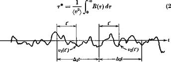
We return now to the condition of statistical independence of adjacent intervals. This implies that the joint probability f(vlt v2) = /(«1)/(«’2) where and »2 are values of the variable during two adjacent intervals and A2t, as illustrated in Fig. 2.14. We saw [following (2.6,30)] that statistical independence implies zero correlation. In the present context we may infer statistical independence from zero correlation. Thus we require that

= «Л = 0 (2.6,53)

DISCUSSION OF CONDITION (ii)

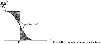
the average being taken over the range 0 <t'< At. Now if we define a characteristic correlation time by

Fie. 2.14

DISCUSSION OF CONDITION (ii)

as illustrated in Fig, 2.15, and require that At t*, then it is evident that condition (2.6,53) will be satisfied. Since the present results will normally be of interest only for large r and large tlt this condition can be met while still keeping n very large. I

ORDINATE-CROSSING RETURN PERIOD

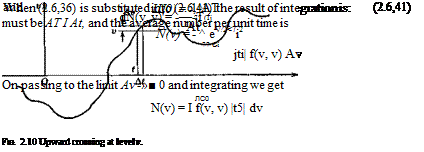
With reference to Fig. 2.10, let us define an “event” as a crossing of the random curve through the strip Av at v. The time At associated with a single event that has a slope in the range Av is

During a total time T —> oo, the portion spent in the domain Av, Av of the (v, v) space is

A T = Tf(v, v) Av Av

ORDINATE-CROSSING RETURN PERIOD

Hence, the total number of events with slopes in the range Av in the time T

ORDINATE-CROSSING RETURN PERIOD

v/ox

Fig. 2.11 Return period.

Since N(v) includes both upward and downward crossings, the average number of upward crossings, or “positive events” is

N+(v) = iN(v) = — ^ (2.6,43)

2ir (Tj

The average interval between positive events is called the return period.

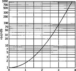
r(v) = —— = 2тг ^ evV2^2 (2.6,44)

N+(v) a2

which is plotted in Fig. 2.11.

DISTRIBUTION OF PEAKS

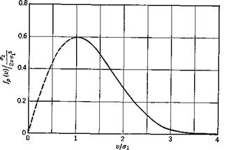
It is observed that for the larger values of v most, but not all, local maxima are immediately preceded by a positive event as defined above. This is illustrated in Fig. 2.4 where the events are defined by the line l. Thus (2.6,43) can also be interpreted as a good approximation to the number of peaks per unit time that are greater than v. It follows that the distribution of peaks per unit time is given approximately by

dv 27t вг

and has the form shown on Fig. 2.12.

ORDINATE-CROSSING RETURN PERIOD

Fig. 2.12 Distribution of peaks per unit time.

PROBABILITY OF A POSITIVE EVENT DURING TIME tx

We now wish to find the probability that a positive event, as defined above, will occur in a given time t^. Let t1 be divided into a sequence of equal intervals At such that the following two conditions are met

(i) At < r(v)

(ii) The probability of an event during any particular interval At is in­dependent of whether an event has occurred in any previous interval. (See below for discussion of this condition.)

Since N+(v) gives the average time density of events, then the probability of an event in At is (for At —> 0)

p(v, At) = AtN+(v) = — (2.6,46)

r(v)

and the probability that there will be no event in At is

q(v, At) = 1— p = 1 — — (2.6,47)

r(v)

Hence the probability that there is no event in n successive intervals is, by virtue of condition (ii) above,

*щШ) = (i-^j)"

If a positive event is identified with “failure” of a system, then clearly q(v, n At) is the probability of “survival”! for a’time tx = n At, i. e.

Подпись:ORDINATE-CROSSING RETURN PERIODПодпись: p{v, tj = 1 - q(v, txORDINATE-CROSSING RETURN PERIOD(2.6,48)

Hence the probability of failure is

(2.6,49)

For large times (the usual practical case) n may be very large and the term in parentheses may be represented by its limit

ORDINATE-CROSSING RETURN PERIOD(2.6,50)

so that the survival probability is

(2.6,51a)

and the failure probability is

Подпись:p(v, tx) = 1 — e~h/r{v)

Подпись: p(v, іг) = 1 — exp Подпись: Jl_ e-»2/2<n2 r(0) Подпись: (2.6,52)

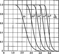
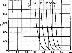
This result is general, and can be applied for any stationary random process. If the process is the Gaussian one previously discussed, then r(v) is given by (2.6,44), and (2.6,516) becomes

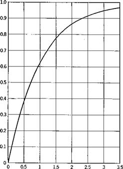
Equations (2.6,516) and (2.6,52) are plotted in Fig. 2.13. It should be noted that the probability of failure associated with t± = r is (1 — 1/e) or 0.63, and that the curves in (6) fall rather steeply over a fairly narrow range of v. Equation (2.6,51a) is a particular case of the Poisson distribution, for zero events in a time tv

f A more rigorous treatment of survival probability covering nonstationary and non-Gaussian processes is given by Rice and Beer (ref. 2.8) and is applied to launch vehicles by Beer and Lennox (ref. 2.9).

p(v, h)


ORDINATE-CROSSING RETURN PERIOD

Ф, h)


v/<7i

(b)


ORDINATE-CROSSING RETURN PERIODORDINATE-CROSSING RETURN PERIOD

ORDINATE-CROSSING RETURN PERIOD

I’M

(e)


Fie. 2.13 Failure probability.

MEAN VALUE OF A FUNCTION OF

Let g(v) be any function of v. Then if we calculate all the values gn associated with all the samples vn(tj) referred to above we can obtain the ensemble

mean (g). Now it is clear that of all the samples the fraction that falls in the infinitesimal range gi <g <9i + Ag corresponding to the range of v vt < v <: v{■ + Av is f(vt) Av. If now we divide the whole range of g into such equal intervals Ag the mean of g is clearly

00

(g) = lim 2,g(f(v{)Av

A u-*0£=l

or (g) = Г g(v)f(v) dv (2.6,27)

J—oo

Equation (2.6,27) is of fundamental importance in the theory of probability.

Подпись: From it there follow at once the formulae for the moments of the distri- butions: <®> = Л00 vf(v) dv = 1st moment of/ J— 00 (2.6,28a) or (®2> = Л00 ®2/(®) 2nd moment of/ (2.6,286) <®n> = Л00 vnf(v) dv = nth moment of/ J—00 (2.6,28c) For the particular case we have been discussing, (v) = 0 and (»2) = «г2.

JOINT PROBABILITY

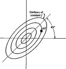
Let vflt) and v2(t) be two random variables, with probability distributions fi(vi) and f2(v2). The joint probability distribution is denoted f(vlt v2), and is defined like f(v). Thus /(iq, v2) AS is the fraction of an infinite ensemble of pairs («j, v2) that fall in the area AS of the vv v2 plane (see Fig. 2.9). If vx and v2 are independent variables, i. e. if the probability j(vx) is not dependent in any way on v2, and vice versa, the joint probability is simply the product of the separate probabilities

/(®i> 4) =/iW/aK) (2.6,29)

From the theorem for the mean, (2.6,27) the correlation of two variables can he related to the joint probability. Thus

Подпись: (2.6,30)B12 = (Vlv2) =jjv1v2f(v1, v2) dvx dv2

— 00

For independent variables, we may use (2.6,29) in (2.6,30) to get

Л oo л oo

^12 = »i/(®i) dv і X V, f(v2) dv,

J— 00 J—oo

= <®l)(®2>

V2

MEAN VALUE OF A FUNCTION OF


Fig. 2.9 Bivariate distribution.

and is zero if either variable has a zero mean. Thus statistical independence imphes zero correlation, although the reverse in not generally true.

The general form for the joint probability of variables that are separately normally distributed, and that are not necessarily independent is

MEAN VALUE OF A FUNCTION OF

(2.6,31)


M = [»%]

ma = («л)

N = [»и] = M-i

For two variables this yields the bivariate normal distribution for which

Подпись: V -®12 -®12 ff22 M

As shown in Fig. 2.9, the principal axes of the figure formed by the contours of constant / for given R(t) are inclined at 45°. The contours themselves are ellipses.

JOINT DISTRIBUTION OF A FUNCTION AND ITS SLOPE

We shall require the joint distribution function f(v, v; 0) for a function v(t) that has a normal distribution. The correlation of v and v is

Подпись: T-oo 2T J-TEvv(t) = Ит ^ f v(t)v(t + t) dt

In particular, when т = 0

1 ҐT A;

MEAN VALUE OF A FUNCTION OF

л*(0) = lim ^ vJ7dt r-co 2T J-t dt

which is zero for a finite stationary variable. It follows therefore from (2.6,33) that f(v, v; 0) reduces to the product form of two statistically independent functions, i. e.

MEAN VALUE OF A FUNCTION OF Подпись: /_ JL _ ЛЛ  2of 2of)

/(»,»; 0) = fx{v) – fiiv)

To evaluate / we need only the two variances. ax = V we have pointed out previously can be found from either i? u(r) or <£>u(ft>). To find a2 = ii we have recourse to the spectral representation (2.6,4), from which it follows that

Л CO

v(t) = imei<oidc (2.6,37)

J CO——CO

From this we deduce that the complex amplitude of a spectral component of v is ico times the amplitude of the same component of v. From (2.6,15) it then follows that the spectrum function for v is related to that for v by

Подпись: (2.6,38)and finally that

(Т22 = (й2) = Ф#(®) dm = (о2Фот(со) dm (2.6,39)

J—CO J—СО

Thus it appears that the basic information required in order to calculate f(v, v) is the power spectral density of v, Ф„„(со). From it we can get both (■v2) and (v2) and hence f(v, v; 0).

The autocorrelation of v can be related simply to that of v as follows. Consider the derivative of R(t)

±nvv(T) = ^<vmt + T)) dr dr

Since the differential and averaging operations are commutative their order may be interchanged to give

j-j; Rw(t) = (v(t) v(t + t)^>

= (v(t)v(t + t)>

Now let (t + r) = u, so that

-7- ^w(r) = (v(u ~ t)v(u)) dr

We now differentiate again at constant u, to get