Category Management and Minimisation of Uncertainties and Errors in Numerical Aerodynamics

Design of the Wing Structure

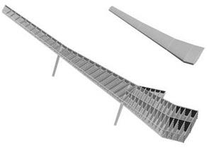
The structure of a common transport aircraft wing is composed of the following components (see fig. 2):

• Spars with spar webs carrying shear load and spar caps which resist tension or compression normal loads. Generally, the wing box is composed of a front and rear spar. The rear spar is of special importance for the mounting of movables as well as for systems integration. As shown in fig. 2, additive components, like a mid-spar, or a false rear spar can be integrated in the wing structure as well.

• Top and bottom covers which have a contouring as well as a load carrying func­tion. These components carry both, normal and shear stresses. Along with main spars, the wing skin forms the box structure of the wing. The skin parts are stiffened by stringers to prevent buckling failure

• Ribs which can be oriented perpendicular to the wing box axis or parallel to the aircraft symmetry plane. Ribs are used to keep the aerodynamic shape of the wing cross-sections under aerodynamic load and for insertion of concentrated loads in the wing box structure caused by engine mountings or landing gear.

In figure 2 different levels of modeling details for each structural component are depicted. The stiffening components, like stringers, spar – or rib caps can be realized by beam elements with defined cross-sections, by rod elements neglecting the bend­ing stiffness of the stiffener or can be "smeared" over the area of the correspondent thin-walled structural component. The smeared stiffening component in turn can be realized as an additional orthotropic material layer, which is reasonable when modeling the skin-stringer panels or taken into account in the wall thickness of the thin-walled components what is commonly done by ribs and spars.

In the current study the structural model is realized by shell and bar elements. The inclusion of element offsets was used as a reference with highest grade of modeling detail limited to the main stiffening components within the present work.

The different levels of detail, shown in figure 2 are employed within the test wing model. The idealized FE models are derived from the reference geometry by repla­cing the built-up structure, realized with shell and bar elements, by a. m. simplified structural design. To estimate the deviations in the deformation behavior caused by modeling simplifications the structural response of both the reference and simplified wing box models is compared for a reference loading. To ensure the comparability of these results the volume of the wing structure was kept constant for all derivations with varying grade of the detail.

Uncertainties caused by different levels of approximation are discussed in the following section. The intent of this overview is not to enable the general prediction
of the modeling error of the structural and thus of the aeroelastic response resulting from distinct simplification. Due to the individual design and stiffness properties of wing structures realized in different aircraft types the contribution of structural components to the bending, shear, and torsional stiffness as well as to the warp­ing characteristics varies depending on a given structural design. Instead of that, a series of calculations is performed to estimate the dimension of the deviations resulting from different levels of simplification using the parametric finite element model. The effect of uncertainty on the stiffness properties of the wing structure is considered only in the frame of static aeroelastic analysis under assumption of lin­ear elastic structural behavior. Non-linear effects as well as dynamic properties or effects caused by the usage of non-isotropic materials are not in the objective of the present work.

Part I: Model Uncertainties

1.2 Introduction

To obtain a high level of accuracy for a structural model one possible approach is to reproduce the real structure with a high level of geometric detail. This approach implies two general drawbacks: it is connected with high modeling effort on the one hand and requires fine discretization of the wing box geometry on the other hand (see Fig. 4, on the left hand side), resulting in high model size and numerical costs. To demonstrate the dimension of complexity connected with a detailed model the reference structure described in section 1.1 is considered. The FE model has 740 design variables and is realized by 24900 shell and 10700 bar elements having in total 260000 degrees of freedom.

For coupled aeroelastic analysis, requiring a high number of iterations the min­imization of the finite element model size could be of high priority. As first ap­proach to reduce the number of degrees of freedom, reduction techniques are used to condense a 3D wing box structural model into a 1D-beam stick model. In the other case, if a parametric FE wing model with variable geometry should be op­timized, the amount of design variables associated with high level of modeling de­tail is undesirable. To reduce the number of design variables a simplified structural model is preferred which is composed only of main components of the wing struc­ture, like top and bottom covers, ribs and spars, including spar caps. Within such simplified models stringer stiffeners are commonly idealized by an additional layer with orthotropic material properties. The next sections deal with the effect of the simplifications within the 3D FE models.

Quantification of Uncertainty

For the quantification of uncertainty affecting the static aeroelastic response differ­ent structural and aerodynamic output parameters are considered. Evaluation cri­teria commonly used for characterization of the aeroelastic response are the lift and drag coefficients for a given angle of attack, natural frequencies, or flutter speed of

the investigated aircraft. In this study only static aeroelasticity is treated, therefore the study is concerned with the aerodynamic performance of an aircraft wing un­der cruise flight conditions (see table 2). For this purpose the converged angle of attack aEqSt is evaluated iteratively for a given lift. A coupled fluid structure ana­lysis is performed using derivates of the wing structural model presented in section

1.1 which is affected by different types of uncertainties. For each derivate relative deviation A aEqSt / aEqSt compared to the result obtained for a reference structure (without modifications) is calculated.

The global values for relative difference to the converged angle of attack A aEqSt / aEqSt presented in this work are influenced not only by the change of struc­tural parameters, but are dominated by the aerodynamic properties of the wing as well as by the given flow conditions and aerodynamic method used within the static aeroelastic analysis. For this reason, the results presented within this work should be considered as sample values to demonstrate the degree of deviation within aero­dynamic output parameters for a special test case.

To examine the change within the wing box stiffness the structural response (without aeroelastic coupling) is calculated for different derivates of the FE test model subjected to a reference load case. The reference load case is represented by a pressure distribution and inertia loads obtained for a reference structure un­der cruise flight conditions. Local values of bending angle w'(y) and twist 0(y) are computed along the structural wing span. These "beam-like" deformations are extracted from the nodal solution of the 3D finite-element model by means of the method presented by Malcolm and Laird [9]. The procedure employs a least squares fitting to extract three translational and three rotational section deformations from the nodal displacements in x-, y – and z-direction for each wing section. This process is applied to a series of sections along the wing span to calculate the bending and tor­sion. For the local values of bending and torsional angle the deviations Aw'(y) and A0(y) are calculated relative to the deformations obtained for the reference struc­tural model. The local deviations are related to the maximum reference values of the corresponding deformation, w'(y)max and 0(y)max respectively. This approach en­sures that no singularities can occur due to very small local values within the torsion deformation.

To estimate the effect of stiffness variation on the wing aerodynamics, a well – known concept for the elastic angle of attack ael is used. This kinematical term describes the local change of the geometric angle of attack ag in flight direction due to elastic deformation of the wing. It affects the load distribution caused by the flexible structure of lifting surface and thus the overall lift coefficient. Deviations in torsion and bending stiffness of the wing box cause a change of the lift distribution over the wing span compared to the reference structure. Under conditions of steady cruise flight this lift change must be corrected by adapting the angle of attack ag of the aircraft iteratively until target lift will be achieved and aEqSt = ag.

For swept wings the local angle ael (y) depends on the torsion deformation 0 (y) as well as on the bending angle W(y):

From the kinematical interrelationship in equation (1) follows that for a wing with positive angle of sweep back ф the torsion and bending contributions of the elastic angle of attack are directed mutually. For this reason, the change of bending angle due to reduction of bending and shear stiffness of the wing box structure can be compensated by the change of torsion deformation caused by the reduced torsion stiffness to a certain degree. For common transonic transport aircraft wing struc­tures the angle ael is dominated by the bending deformation and for this reason is negative.

To estimate the effect of the variation of torsion and bending distortions on the deviation of the elastic angle the propagation of uncertainty is applied on equation

(1)

Quantification of Uncertainty Quantification of Uncertainty Подпись: sin ф(у) (2)

. For a local relative deviation A ael (y)/a^ in elastic angle of attack a mathem­atical correlation (2) is the following:

The local values A0(y)/0max and Aw'(y)/w’max are relative deviations of tor­sion and bending distortions due to the local change of wing box stiffness caused by different degrees of modeling simplification. These values are structural parameters depending on the stiffness properties of the structure. The terms 0max/a^ cos ф and w’max/aeax sin ф in equation (2) are ratios of the local torsional and bending angles relative to the maximum value of elastic angle of attack. These values de­pend on the local sweep back angle ф(у) of the wing box reference axis, the load distribution in chord and span-wise directions (ratio of the distributed moment relat­ive to the distributed load) as well as on the ratio of the torsion stiffness GJ relative to the bending stiffness EI.

The local deviations of the elastic angle of attack A ael (y) / aeax are related to the maximum value obtained for the reference FE model in the same manner like deviations of structural deformations. Since the effect of the deviation of this para­meter on the geometric angle of attack ag and thus on the local lift distribution is depending on the magnitude of ael (y) this approach seems to be more suitable for the objective of the present study than relating this term to the reference local values as commonly done. The latter method would overestimate the influence of the deviation A ael (y) considering local variations of the elastic angle of attack near the root as well, which have no appreciable effect on the load distribution due to the very small values of ael (y) within this area.

Quantification of Uncertainty Подпись: (3)

The distribution of the local deviations A0(y)/0max, Aw'(y)/w’max and A ael (y) / a<miax varies along the wing structural axis, depending on the stiffness and load distribution of the present wing structure and aerodynamic design. To obtain global deviation parameters the mean values of these local variations are calculated in sections using a relation defined exemplary in equation (3) for the bending angle:

where з is the structural span of the wing box. Mean values of twist [AQ] and elastic angle of attack [Aael ] are obtained in the same way. To assess the contri­bution of the variations of torsional and bending angles to the deviation of elastic angle of attack, the local values Aw'(y)/w’max and AQ(y)/Qmax, multiplied with the parameters’ terms w’max/aeJlca sin ф and Qmax/a^cosф from equation (2), are integrated by means of eq.(3). These "transformed" values [Aw’]/r and [AQ}tr are also used within the present work to estimate the effect of variation within struc­tural stiffness properties caused by modeling or stochastic uncertainties on the load distribution. The difference between the term [Aael] = [AQ}tr — [Aw’]tr calculated from the global bending and torsion deformations and the mean value resulting from integration of the local values A ael (y) / a^ directly obtained from the structural response is between 0.01% and 0.03%.

Because nonlinear behavior of aeroelastic problems is highly depending on the local flow conditions as well as on local stiffness characteristics of the wing struc­ture, the change in equilibrium state angle of attack A aEqSt / aEqSt cannot be pre­dicted using a mean value [Aael ] for a complex structure in a direct way. Never­theless, as will be shown within the following sections, the parameter [Aael ] is a suitable indicator to estimate the deviation tendency of wing aerodynamics due to the variation within the stiffness properties of the wing.

Finite Element Models and Analysis Methods Used for Uncertainty Quantification

1.1 Parametric Finite Element Model

A code already developed at the Institute of Aircraft Design and Lightweight Struc­tures (IFL) is enhanced to generate a finite element model of the structure. It is based on the parametric description of airplane wing geometry and a layout of the load-bearing structure [1], [2]. The code is written in Patran Command Language (PCL) which allows an automated generation of finite element wing models by the preprocessor MSC Patrano.

A HIRENASD wind tunnel model [3] scaled up to 58 m of span is employed as a test structure for investigations carried out in the context of the MUNA project. The wing box structural layout and the arrangement of engines are taken on from the predecessing project [4] and resemble the wing of an AIRBUS A340 aircraft (see Fig. 1).

The geometric data are imported from an ASCII input file and are employed to generate a finite element shell model of the wing. A transonic transport aircraft design is used with the corresponding weights given in table 1 to evaluate the target lift for the calculation of aerodynamic and static inertial loads.

Due to a high number of required aeroelastic calculations, especially for the stochastic analysis presented in the second part of the work, the high order panel method HISSS is used instead of an Euler or RANS code to calculate the discrete aerodynamic nodal loads. The lack of accuracy when calculating a load distribution on the wing surface at higher Mach numbers had to be accepted so that the numeric costs could be kept reasonable. The finite-element solver NASTRAN was used to calculate the nodal displacements of the structural model.

The in-house code coupling library ifls [5] was employed to perform the fluid – structure interaction. The code handles the load and displacement transfer between non-conform grids by using a three-field approach in combination with Lagrange multipliers. The structure of the coupling routine allows the interaction between dif­ferent commercial numerical solvers. The converged angle of attack aEqSt of static aeroelastic equilibrium was estimated by ifls iteratively for given lift and flow con­ditions by variation of an overall (geometric) angle of attack ag of the wing.

Table 1 Weights for the transonic transport aircraft design used in this study

Gross weight

mTOW

to

256

Fuselage and empennage unit structure + payload

тЕр + m-N

to

95

Wing structure

mw

to

35

Total fuel mass

mp

to

106

Propulsion group

mpG

to

20

Finite Element Models and Analysis Methods Used for Uncertainty Quantification

Fig. 1 HIRENASD wing geometry and structural layout

Nodal loads calculated on the aerodynamic surface were transferred to the nodes of the structural grid by means of conservative interpolation in the area of the wing box. In the region of the flap and slat structure the aerodynamic nodal loads were applied to additionally created auxiliary structural nodes and tied to the wing box by multi point constraints of RBE3 type.

The static inertial loads including fuel weight, engine loads and the weight of the flap structure had also to be taken into account to represent realistic loading conditions. The flap and slat structure were idealized as point masses and connected to the spar structure by multi point constraints in the same way as the aerodynamic forces. The masses of the high lift devices were also required for this idealization and were estimated by handbook methods [6]. Tank loads were also modeled with point masses and RBE3s. The tank masses were evaluated for each wing bay by calculation of the volume taken by the fuel for a given degree of refueling.

The static inertial loads including fuel weight, engine loads and the weight of the flap structure had also to be taken into account to generate realistic load cases. The flap and slat structure were idealized as point masses and tied to the spar structure by multi point constraints in the same way as the aerodynamic forces. The masses of the high lift devices needed for this simplified approach were estimated by handbook methods [6]. Tank loads were also modeled with point masses and RBE3s. The tank mass was estimated for each wing bay by calculation of the volume taken by the fuel for a given degree of refuelling.

The wing box structure was sized with respect to strength criteria and constraints of buckling stability. Two load cases were selected for the sizing process: a 2,5g maneuver and the landing impact (see table 1). The strength sizing was carried out by a fully stressed design using stress distribution computed for limit loads and a yield-stress criterion. The design against buckling failure was performed by hand­book methods [7] using maximal allowable stresses for the compression panels

Table 2 Weights for the transonic transport aircraft design used in this study

2.5g maneuver

Altitude

H

km

11

Mach number

Ma

0.82

Gross weight

mrow

to

256

landing impact

Altitude

H

km

0

Mach number

Ma

0.2

Gross weight

mrow

to

182

Cruise flight (1g) Altitude

H

km

11

Mach number

Ma

0.82

Gross weight

mrow

to

256

as well as optimum design curves and semi-empirical formulas for estimation of stiffener spacing and cross-section geometry.

Due to constraints defining the highest permitted elastic deflection of the wing tip given in [4], the wing box was also sized under consideration of stiffness. For this additional sizing procedure the contribution of structural members to the wing deflection was calculated following the pattern of the modified fully utilized design method (MFUD) proposed by Patnaik et al [8]. For the constrained degree of free­dom (in this case it is the bending displacement) the sensitivity factors can be cal­culated for each component of the structure. These factors are defined as dw/dm where dw is a partial change of displacement and dm is a change of structural mass. The change of bending deformation and structural mass are evaluated by attach­ing additional material (by increasing wing thickness or stiffener cross-section) to each structural member and recalculating the displacement w of the modified struc­ture subjected to a reference load case. These sensitivity factors are used within the MFUD-procedure to weigh the increase of wall thickness of the structural members until the displacement constraint is achieved. This method permits to attach an addi­tional structural mass only in those areas of the wing box whose stiffness influences the given deformation at most. The weight of the structure sized with this approach was estimated to be very close to those obtained by a time-consuming optimization procedure [8].

Uncertainties of Numerical Structural Models in the Frame of Aeroelasticity

P. Reich, A. Reim, M. Haupt, and P. Horst

Abstract. Today, numerical methods for structural and aerodynamic problems are reaching highly versatile and reliable levels. Therefore, the coupling of both do­mains can be solved at a high standard. On the other side, the accuracy of aeroelastic analyses depends on the level of precision with which the stiffness properties and, thus the structural behavior of an aircraft wing structure in means of deformation can be predicted. The presence of uncertainties within the structural model which is in­tegrated in the coupled analysis can affect the fidelity of the structural response and, thus, influence the results of the numeric aerodynamic simulation as well. Invest­igations carried out by the Institute of Aircraft Design and Lightweight Structures (IFL) in the frame of the MUNA-project were focused on two types of uncertainties affecting the accuracy of the static aeroelastic analysis: stochastic uncertainties and uncertainties due to modeling simplifications. Stochastic uncertainties are caused by the deviation of actual structural parameters in realized aircraft wings, like Young’s modulus or wall thicknesses from the original ideal design. This deviations affect the stiffness of the real structure and, thus the structural and aerodynamic response. A method to estimate the sensitivity of the wing structure to random input paramet­ers is presented in the second part. The second class of uncertainties arises from approximations connected to the idealization of the physical and geometric proper­ties of the real structure used in finite element (FE) structural models. In the first part of this work, an overview of modeling effects is given which affect the stiffness properties of the FE structural models and in turn influence the results of static aer- oelastic analysis. The coupled analysis is carried out with a high-order panel method for the aerodynamic domain and a parametric finite element structural model, which allows a wide variation of material and geometric properties of wing box structure. This structural model as well as the aerodynamic method and the coupling routines are presented in the following section.

P. Reich, A. Reim, M. Haupt, and P. Horst

IFL, Hermann-Blenk-Str. 35, D-38108 Braunschweig

e-mail: paul. reich@tu-bs. de

B. Eisfeld et al. (Eds.): Management & Minimisation of Uncert. & Errors, NNFM 122, pp. 157-180. DOI: 10.1007/978-3-642-36185-2_7 © Springer-Verlag Berlin Heidelberg 2013

Laminar Boundary Layer at High Reynolds Number

For the second application we solve the compressible Navier-Stokes equations at a low Mach number for a classical test case, the flow over a flat plate. We are simu­lating a laminar boundary layer but for a very high high Reynold number. Ludwig Prandtl and Blasius, one of his students, made pioneering achievements with their work on the boundary layer. This ended up in the solution of Prandtl’s boundary layer approximation equations by Blasius, reducing them to a nonlinear ordinary differential equation (ODE) of third order for the case of a laminar steady flow. This ODE can be solved nowadays numerically by a math algebra program with an arbitrary accuracy. We employed the software Matlab where we solved Blasius’ boundary layer equations (see e. g. [16]) with a four step Runge-Kutta scheme and a Newton-Raphson iteration method. This serves us as the reference solution for the iterated defect correction applied on the Navier-Stokes equations.

To point out the abilities of the WENO reconstruction in a reference space used in our work and the approach of the iterated defect correction we still used a fully unstructured triangular grid even in the boundary layer. For a finite volume scheme, this is a quite demanding task where surely some extra fine tuning is necessary to obtain satisfying results. One of them turned out to be the numerical flux approxim­ation for which we took the HLLC flux as described in [20]. Our computational do­main is Q = [-0.5,2]x[0,0.05] discretized by a total of 5250 triangular elements. In the interval -0.5 < x < 0 we use a slip wall boundary condition where the velocity normal to the wall is zero. At x = 0 we impose than a non-slip wall adiabatic bound­ary condition in the interval 0 < x < 2. The free stream Mach number is Ma«, = 0.3, resulting from the free stream flow parallel to the wall with u«, = 0.3, p«, = 1 and p«, = 1 /у. As we use the equation of state for ideal gas the ratio of the specific heats is у = 1.4, whereas the Prandtl number is Pr = 1.

Подпись: 0.02 0.018
Laminar Boundary Layer at High Reynolds Number

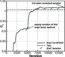
Fig. 7 Lift (left) and drag (right) coefficient computed with a first order basic method and a 3rd order defect reconstruction, compared with a second order TAU code solution on the same grid

For the chosen high Reynolds number of Re = 106 [1/m] we set our viscosity to д = 3 • 10-7 making again the assumption of a constant viscosity in the whole domain. To resolve the flow at high Reynolds numbers, which implies a very thin boundary layer of 5X=1 = 5 • 10-3 in our case, a highly stretched grid in the boundary layer is necessary. At v = 1 we therefore have cells with an aspect ratio of 1 : 205. However the chosen spacing at the first cell of y1 = 4 • 10-4 is still quite high com­pared to setups in the literature which are meant to be solved with a finite volume method 2nd order TVD method (see e. g. [9]). In addition we use only 8-9 cells to discretize the boundary layer at v = 1.

Laminar Boundary Layer at High Reynolds Number Laminar Boundary Layer at High Reynolds Number

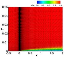
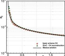
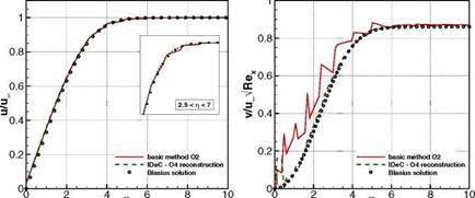
The initial condition is given by the free steam conditions and we take a homo­geneous block profile with the free stream conditions at the inflow. It is important that mass can escape at the farfield, since due to the boundary layer growth we get a non-zero velocity outwards. At the outflow we can use simple extrapolation of the inner state values and impose only the free stream pressure. For the computation we used a second order basic scheme to obtain a steady solution which we reach after t = 20 seconds of simulation time. After each steady solution we apply the defect correction with a 4th order accurate WENO reconstruction again with the paramet­ers ne = 2L, r = 6, £ = 10-14 and Xc = 105. Left in Fig. 8 we see the distribution of the dimensionless x-velocity u/u^ in the whole domain for the basic method. In addition we compare the Blasius solution with the velocity profiles of both u and v components of the velocity at the position v = 0.7 (see Fig. 9) and with the skin friction coefficient over the entire plate (see Fig. 8, right). For all comparisons the corrected numerical solution, here shown after four defect correction iterations, is in good agreement with the Blasius reference solution. At this point, we have to men­tion, that using a scheme of higher order with WENO reconstruction is unstable and

Fig. 8 Flat plate at high Reynolds number Re = 106 [1/m] with a = 0° and Ma = 0.3 com­puted with a 2nd order basic method and corrected using a 4th order WENO reconstruction. Left we show the distribution of the dimensionless x-velocity u/u^ in the whole computa­tional domain and right the skin friction coefficient is depicted over the plate length after four defect correction iterations.

Laminar Boundary Layer at High Reynolds Number

Fig. 9 Flat plate at high Reynolds number Re = 106 [1 /m] with a = 0 and Ma = 0.3 com­puted with a 2nd order basic method and corrected using a 4th order WENO reconstruction. Distribution of the dimensionless x-velocity u/uM (left) and of the dimensionless y-velocity v/u^-/Re^ (right).

no steady solution can be obtained. The method of iterated defect correction seems to be stable, as it is based only on a second order scheme, and is nevertheless able to correct the basic method with the high order accurate defect.

For the и component we can see in the zoom made in the section of the dimensionless variable 2.5 < t] < 7 with t] =y/y^p and the kinematic viscosity

v = р/р, that we get a smoother distribution by applying the defect correction. In the case of the dimensionless v component of the velocity v/iioo/Rex with Rex = the improvement of the solution is considerable. The completely wrong distribution of the basic method could be corrected to fit quite well with the reference Blasius solution. Near the wall we nevertheless reach the limits of the re­construction, which has shown so far that the reconstruction in the reference space can cope even with these highly stretched elements. The corrected skin friction coef – flcient (Fig. 8, right) shows also better agreement with the reference solution espe­cially at the beginning and the end of the plate. The remaining difference is due to the stagnation point at x = 0 where high gradients occur, causing oscillations. As can be read in literature the prediction of skin friction coefficients still remain a difficult issue in the numerical simulation. Similar to [9] we compare therefore the friction coefficients at the end of the plate at x = 2. The analytical solution can again be computed by solving the Blasius equations and we get

0.664 pu^x

cf=—F= with Rex=———————————— . (41)

/Rex P

With Cf (x = 2) = 4.983 • 10~3 the error of the skin friction of the basic method is of 6.1% and with the iterated defect correction approach it could be corrected to Cf (x = 2) = 4.653 • 10~3 resulting in a remaining error of 0.9% for this case.

1.2 Conclusion

In this work we applied the method of iterated defect correction to a finite volume scheme and solved both, the Euler and the Navier-Stokes equations. A steady solution of lower accuracy, mostly of first or second order, is the starting point for the method of iterated defect correction. The next step consists of a WENO recon­struction which is used to evaluate the local defect of the steady solution. If we modify our equations by putting the local defect on the right hand side as a negative source term, the low order solution can be iteratively shifted to the accuracy of the reconstruction. The main advantage of this approach is that the high order scheme has not to be solved – the high order scheme is only used to calculate an estimation of the local discretization error. Hence, this approach can be used to increase the accuracy of an existing code in a straightforward way. It seems that the high order approximation also inherits some additional stability from the low order solver. Our results show that the iterated defect correctionin combination with the WENO re­construction in [4] for unstructured meshes works very well. We did not succeed to define robust boundary conditions in any case. This seems to be even more subtle than the definition of high order boundary conditions in general.

We have shown numerical convergence results up to sixth order of accuracy, ap­plying the method of iterated defect correction starting with a first order steady solution. By modifying the original approach, a relevant speed up could addition­ally be achieved for equations with source terms depending on the solution itself. The scheme remained stable even for the more challenging test case of the transi­ent Ringleb’s flow. A fourth order accurate solution could be achieved here from a first order numerical scheme. Convergence studies using the manufactured solu­tions method have shown that in the case of the Navier-Stokes equations, where a local defect can be computed separately for the convective and the diffusive fluxes, it is crucial for flows with low Reynolds numbers to evaluate the local defect for all fluxes. Neglecting the defect in the convective fluxes still gave better absolute error norms compared to the low order solution, but the expected high order of the reconstruction was not reached for our test cases.

A RAE 2822 profile have been computed as an application test case, solving the Euler equations with a first order basic scheme applying a third order accurate re­construction to determine the local defect. Compared to the first order solution the aerodynamic coefficients like lift and drag could be corrected by 11%, respectively 28%. As a second application test case a laminar boundary layer at a high Reynolds number of Re = 106 was numerically solved using the iterated defect correction. Better results compared with the second order starting solution could be achieved applying the defect correction combined with a fourth order reconstruction. For ex­ample a reduction of the skin friction error at the end of the plate from 6.1% with the basic scheme to 0.9% was reached in this case.

Application Test Cases

1.1.1 The RAE 2822 Profile

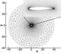
As a first application test case for the method of iterated defect correction we sim­ulated the flow around the RAE 2822 profile in two dimensions. It is one of the official test cases of the project MUNA. We solve only the nonlinear Euler equa­tions for this test case, so the grid we used is fully unstructured and contains about

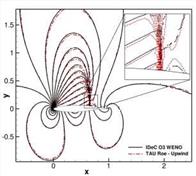
18.0 elements with a relatively high discretized profile of 180 points per each half of the profile. The farfield is situated at 40 cord lengths and the profile is simulated as slip wall with the velocity normal to the wall set to zero. The flow was defined by the flow conditions of the so-called test case 9 with Ma = 0.73 and an incident angle a = 2.78°. This yields a transonic flow with a shock on the upper side of the pro­file (see Fig. 6, right). To compare the solution of the iterated defect correction we performed the simulation on the same grid with the numerical code of the DLR

Application Test Cases

Fig. 6 Fully unstructured grid for the RAE 2822 profile (left) and Mach number distribution of the corrected solution and a direct solution with the TAU code using a second order TVD upwind scheme (right)

("Deutsches Zentrum fur Luft – und Raumfahrt"), the TAU code, used as standard code for the project MUNA. The parameters for the TAU code were set to a second order TVD scheme with a least squares reconstruction and the Roe approximation for the convective flux.

In the case of iterated defect correction we used a first order basic method and corrected the steady solution by a local defect reconstructed with the WENO method described in section 3 using polynomials of degree two. The difference between the basic method and the corrected solution can be seen for the aerodynamic coeffi­cients. In Fig. 7 we show the lift and drag coefficients over the number of iterations. Our iterative method is a rather suboptimal explicit method and so the number of iterations needed for a steady solution is quite high but does not influence the defect correction and is not of interest here. When the solution does not change any more we compute the local defect and solve afterwards the modified equations (5) to ob­tain a corrected solution which is denoted by the small arrows in Fig. 7. So each small arrow stands for a defect correction iteration.

We can see that the lift coefficient could already be corrected to the end solution after just one defect correction, whereas the drag coefficient needs some more defect correction iterations to converge. In the case of the lift coefficient a correction of about 11% was obtained and the drag coefficient could be corrected with even 28% of the first order solution, what corresponds to a total reduction of around 80 drag counts. The results of the TAU code serve here not only for validation but as a comparison as well, not having an exact solution for this test case.

In addition to the aerodynamic coefficients we can clearly see that by the iterated defect correction method with a 3rd order WENO reconstruction the shock is better resolved than it is with the second order least squares in the TAU code (see Fig. 6, right). Only if we once adapt the grid globally we are able to reach approximately the same shock resolution with the second order scheme.

Numerical Results

For the validation of the implemented iterated defect correction method exhaust­ive studies have been made for 1D, 2D and 3D Euler and Navier-Stokes problems. All simulations have been carried out with a standard finite volume scheme using ghost cells to impose boundary conditions. Depending on the test case a first or a second order basic scheme was used, whereas for the defect correction a polynomial WENO reconstruction up to 6th order was applied with the standard choice for the reconstruction parameters shown in section 3. In this section we first show some of the convergence studies of those validation cases and we end up with application test cases.

1.1 Convergence Studies

To validate our proposed iterated defect correction method for inhomogeneous prob­lems we took as a first example in 1D the nonlinear Euler equations where a source term s(u, A), depending on the solution u and a given geometry A, was added. The equations in (29) are derived from the homogeneous Euler equations in three di­mensions with the assumption of a continuous area variation (see also [20]).

1 ( PuAx

u,+F(u).x- = s(u) with s = —— I p/rA. v (29)

u(e + p)AxJ

This gives an approximation of a 2D axi-symmetric nozzle flow with the x-axis as nozzle symmetry and A(x) as cross-sectional area along the nozzle. In our case we took a smooth sinus function

( 2, — 1 < x < — 2

A(x) = < 2 — sin4 (я(х+ ^)), — ^ < x < ^ (30)

1 2, 2 < x < 1

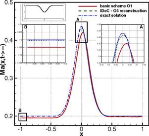
for the cross-sectional area which is illustrated in the upper left corner of Fig. 1. We took a subsonic expansion with inflow and outflow pressure p = 1 and an inflow velocity u = 0.2 with an inflow mass flow pu = 0.28. We obtain then an inflow Mach number of Ma = 0.2 which can be introduced into the 1D nozzle theory to evaluate the exact state at the inflow and outflow section. This is imposed during the simulations which result into a symmetrical distribution of the state variables (see Fig. 1). We can clearly see the difference between the first order basic method and the corrected solution in both amplitude and location of the peak which is expected to be in the nozzle throat at x = 0. In this case a cubic polynomial reconstruction was chosen to compute the local defect.

To measure the exact error between the approximated solution uh and the exact solution ue we use continuous Lp norms

Numerical Results

Fig. 1 Mach number distribution of a axi-symmetric nozzle flow simulated with a first or­der basic method and corrected by a fourth order polynomial reconstruction for the local defect

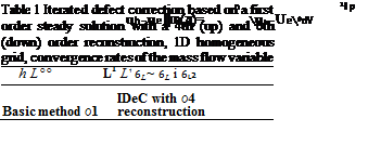
whereas the L“-norm gives the maximum absolute error arising in the whole do­main. We compute the integral with the Gaussian quadrature algorithm with twice the number of Gauss points compared to the numerical scheme. For the defect cor­rection it is important to make this analysis with the high order polynomials and, respectively, with the high order integration and not with the accuracy of the ba­sic method. Table 1 shows the convergence tables of the nozzle test case for five successively refined grids. In addition to the fourth order defect reconstruction we show a convergence table for a first order basic method corrected with a 6th order reconstruction to determine the local defect.

The validation of the 2D and 3D implementation has been carried out by using the method of manufactured solutions, i. e. we insert an analytical function

pe(x) = sin(nx) ■ sin(ny) + 2

for the exact density distribution in 2D and respectively

pe(x) = sin(nx) ■ sin(ny) ■ sin(nz) + 1

in 3D into the Euler equations and solve the inhomogeneous two-, respectively three-dimensional Euler equations

Numerical Results
Подпись: (31)

U + V ■ F(u)= s(x). (32)

0.080 7.69E-03 2.17E-03 2.64E-03

0.040 6.34E-04 1.26E-04 1.78E-04

3.6

4.1

3.9

0.020 3.46E-05 6.08E-05 9.69E-05

4.2

4.4

4.2

0.010 2.14E-06 3.19E-06 5.63E-06

4.0

4.3

4.1

0.005 1.35E-07 1.83E-07 3.44E-07

4.0

4.1

4.0

Basic method 61 —t IDeC with 66

reconstruction

0.100 8.80E-03 2.22E-03 2.49E-03

0.067 1.92E-03 2.95E-04 4.19E-04

3.8

5.0

4.4

0.033 6.66E-05 8.94E-06 1.54E-05

4.9

5.0

4.8

0.017 1.54E-06 1.80E-07 3.28E-07

5.4

5.6

5.6

0.008 2.63E-08 3.02E-09 5.58E-09

5.9

5.9

5.9

The remaining state variables like the velocity and the pressure were set to a constant value greater zero. For our choice we obtain source terms which in contrast to the one dimensional analysis depend only on the space

Si = n ■ sin(nx) ■ cos(ny) + n – cos(nx) ■ sin(ny) for i = 1…4 (33)

in two dimensions and respectively

si = п■ sin(nx) ■ sin(ny) ■ cos(nz) + п ■ sin(nx) ■ cos(ny) ■ sin(nz)

+ п ■ cos(nx) ■ sin(ny) ■ sin(nz) for i = 1…4

3п 3п

Ss = — • sin(jtx) ■ sin(jty) ■ cos(jtz) + — ■ sin(jtx) ■ cos(jty) ■ sin(jtz)

3п

+ — ■ cos(jtx) ■ sin(jty) ■ sin(jtz) (34)

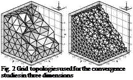
in three dimensions. For the simulations we initialized the domain Q2D = [0; 1]x[0; 1] in 2D and respectively Q3D = [0; 1]3 in 3D with the exact solution and iterated the basic scheme to a steady state with the exact solution imposed on the boundaries. The same convergence study as in one dimension based on the L^-norms was car­ried out on four successively adapted grids. In all our computations we used fully unstructured grids with irregular triangles in two dimensions and tetrahedrons in three dimensions. Each adaptation is performed globally, i. e. we applied the so – called red-refinement in each cell of the domain per adaptation step. An example of two adaptation steps is shown for the three dimensional case in Fig. 2.
Numerical Results

Again we can see the difference between the solution of the basic method and the corrected one. This is demonstrated for the two dimensional case for the density distribution in Fig. 3. We have to mention that for the visualization of the higher order solutions we subdivide the numerical grid and write out the value of the poly­nomial distribution at each barycenter center of the subdivided grid. In this way we can see the Godunov approach of constant values in the cell for the first order solution (Fig. 3, left) and the continuous fourth order solution with vanishing jumps between the cells (Fig. 3, right). A quantitative analysis can be done by determining the convergence rates for the corrected solutions as it was done in the one dimen­sional case. In Tab. 2 we show the experimental convergence order for the two – and

Z

Подпись:Numerical ResultsПодпись: Z X Y

X Y

p: 1.9 2.1 2.3 2.5 2.7 2.9

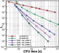
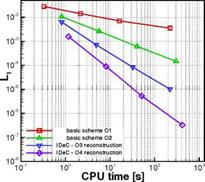
Fig. 3 Solution of the first order basic scheme (left) and the corrected solution of an IDeC with a 4th order polynomial reconstruction for the local defect (right) three dimensional simulations where we used a first order basic scheme with a cu­bic polynomial reconstruction for the defect correction. In both cases we reach the optimal theoretical convergence order of M + 1 when iterated defect correctionis applied. The convergence rates can approve that with the mesh step size h ^ 0 the error tends towards zero with the potential power of M + 1, M being the polyno­mial degree of the reconstruction basis polynomials W (see chapter 3). However, nothing can be said about the real simulation time needed by the employed nu­merical scheme and with it the real gain of using a higher order reconstruction. Therefore we show in Fig. 4 the L1-norm of the errors for the one and two dimen­sional computations described above over the total CPU-time in seconds needed

Table 2 Density convergence rates for IDeC with a first order basic scheme and a cubic polynomial reconstruction on 2D (up) and 3D (down) irregular unstructured grids)

h U° Iі Lr 6L~ 6Li ^7

2D Basic scheme O1 ^ IDeC with O4 reconstruction 0.191 7.55E-02 1.06E-02 1.45E-02 – – –

0.096 5.78E-03 4.68E-04 7.12E-04 3.7 4.5 4.4

0.048 7.07E-04 2.95E-05 4.91E-05 3.0 4.0 3.9

0.024 4.97E-05 1.69E-06 3.17E-06 3.8 4.1 3.9

3D Basic scheme &Л —t IDeC with 6‘4 reconstruction 0.182 5.67E-02 9.49E-03 1.22E-02 – – –

0.127 9.69E-03 1.87E-03 2.39E-03 5.0 4.6 4.6

0.068 8.71E-04 1.01E-04 1.32E-04 3.8 4.6 4.6

0.035 8.38E-05 7.09E-06 9.54E-06 3.6 4.1 4.0

Numerical Results
Numerical Results

Fig. 4 Convergence rates over total CPU time for first and second order methods compared to iterated defect correction with higher order reconstruction in 1D (left) and 2D (right)

for a converged iterated defect correction and the basic schemes of first and second order. The simulations were all performed on one single AMD Athlon 5200+ pro­cessor with 3GB of RAM. So we can compare directly the computational effort to reach the same given accuracy of the L1-norm. To give an example, if we want to reach an error norm of L1 = 10-4 in the one dimensional case (Fig.4, left), we obtain a speed up of factor 4 comparing a second order scheme with a third order corrected solution based on a first order basic scheme. The same comparison for the two dimensional case leads even to a speed up of factor 20 which is due to higher computational cost for the 2D simulations concerning for example the integration (Fig.4, right). This results for the speed up are surely dependent on the test case, nevertheless they give an idea of the potential of higher order schemes. However, in the one dimensional test case we can see, that the speed up of a higher order scheme starts to be significant for very low accuracy levels.

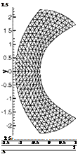
A more demanding test case for the stability and the convergence of the iterated defect correction for the steady nonlinear Euler equations is the Ringleb’s flow [2]. It is one of the few continuous transonic flows of a blunt obstacle which can be solved analytically with the Hodograph method in a transformed (V – 9) plane, with V as the velocity magnitude and 9 the angle of the velocity with respect to x-axis. More details on the Hodograph method and the analytical solution can be found in [2]. In our case the flow direction is upwards with the wall boundaries left and right. Their topology is derived from the analytical solution where the chosen boundaries of our test case represent two stream lines. The inflow and outflow boundaries are circles also given by the exact solution. The chosen geometry leans on th article [21].

In spite of being a transonic flow, it is smooth in the whole domain and since we can compute an exact solution at each grid point there is also a quantitative analysis possible. In addition the flow is supposed to be irrotational and isentropic. We performed the simulations on three successively adapted regular triangular grids imposing the exact solution on every boundary. Starting from the exact solution as

Подпись: 2.5 _2 5г -1.5 -1 -0.5 0 0.5 1 1.5 X Numerical Results Numerical Results

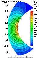
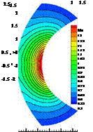
Fig. 5 One of the used triangular grids, steady solution of the first order basic method (middle) and defect correction solution with 4th order reconstruction (right)

the initial condition we use a first order scheme as the basic method for the iteration to a steady solution. In Fig. 5 the middle fine grid is depicted together with the steady solution of the basic method and the solution corrected with IDeC. We expect a complete symmetrical solution with a defined circular sonic line. The first order basic method clearly failures in these flow topologies. There are small instabilities, nevertheless the method is stable and converges perfectly, which is important for the method of iterated defect correction. For the defect correction we applied a 4th order accurate WENO reconstruction with the parameters ne = 2L, r = 6, є = 10“14 and Xc = 105.

With the IDeC we get a good solution which is near to the exact one in spite of the unsymmetrical solution of the basic method. With this setup we reach the theoretical convergence order of the reconstruction, proving the possibilities of the iterated defect correction method. If we compare the absolute error Lp-norms (Tab. 3) of both solutions this means a correction of the basic scheme from one up to four orders of magnitude for the finest grid.

Beside the nonlinear Euler equations we applied the method of iterated defect correction on the Navier-Stokes equations as well. Similar to the convergence stud­ies shown before, we used the method of manufactured solution and solved

ut + V • F(u, Vu) = s(x) (35)

with F(u, Vu) =Fc(u) — Fd (u, Vu), where Fc and Fd denote the convective respect­ively the diffusive flux. The defect correction formulation in (11) does not change in the case of solving the Navier-Stokes equation, but is just extended by the diffusive flux what results in

N

L°°

z7

Lr

6l~

6Li

6L2

Basic method 6‘ 1

32

5.55E-02

5.89E-02

3.68E-02

64

3.56E-02

3.14E-02

2.01E-02

0.9

0.9

0.6

128

2.20E-02

1.64E-02

E06E-02

0.9

0.9

0.7

Basic method

61 —г IDeC with 64 reconstruction

32

4.17E-03

9.55E-04

8.10E-04

64

3.23E-04

4.10E-05

4.04E-05

3.7

4.5

4.3

128

1.90E-05

2.07E-06

2.04E-06

4.1

4.3

4.3

Table 3 Convergence rates for the first order basic method (up) and the corrected solution with 4th order reconstruction (down)

Подпись: with Подпись: ndS'r Подпись: w Подпись: n Подпись: SK Подпись: (37)

with Qi still acting as a placeholder for uf «f+1] and wf]. Similar to the Euler equations the local defect is now computed for both fluxes, the convective and the diffusive flux. A high order formulation for the diffusive flux is therefore necessary. We have chosen the approximation suggested by Gassner et al. in [8]. It enables a one-step numerical method of high order accuracy in space and time using the same data as for the convection flux. Based on the idea of Godunov for advection problems not with constant initial data but with a linear initial distribution, it res­ults in the so-called diffusive generalized Riemann problem (dGRP). Solving this Riemann problem yields two parts, the one containing the arithmetic mean value of the first derivative, whereas the second contains a physically motivated limiting term composed of the jump in the state of two adjacent cells. In 2D and 3D this leads to

a numerical approximation for the diffusion flux, d/dn denoting the derivative in normal direction. The characteristic length h is taken as twice the distance from the barycenter of the cell Ci to the barycenter of the edge K of the computed flux. The integration is again done by Gaussian quadrature with o)K the weights on the edge K using a total number nGP of integration points. The jump in the state of two neighboring cells is multiplied by the parameter n

П = —)= (39)

hJ n

which can also be interpreted as a penalty term for the jump. With the chosen WENO reconstruction we obtain the derivative directly from the reconstructed polynomial distribution. However, the theoretical convergence order for this flux is limited to M, the degree of the reconstruction polynomials, in the case of a finite volume method. This is due to the fact that we use the first derivation of our polynomials losing hence one order of accuracy (see also [8]).

As an exact solution for the iterated defect correction applied on the Navier – Stokes equations simulated in two dimensions we took

Подпись: (40)Подпись:sin(nx)sin(ny) + 4 sin(nx)sin(ny) + 4 sin(nx)sin(ny) + 4 (sin(nx)sin(ny) + 4)2

with u = (p, pu, pv, pe)T denoting the vector of the conservative state. By inserting (40) into (35) we can again compute the source term s, which is only a function of the space x. To test the method of iterated defect correction for rather viscous flows we chose a viscosity д = 10~ which results in a very low Reynolds number of Re = 80. As the temperatures are very low and do not take effect on the viscosity, we performed these computations with the assumption of a constant д. The simula­tions were all carried out on a fully periodic domain Q = [0;2]x[0;2] with periodic boundaries on successively adapted regular triangular grids.

As we use the derivative of the polynomial distribution for the flux approxima­tion we have to take a basis scheme with at least second order of accuracy for the defect correction. In Tab. 4 we show the convergence rates of the test case above computed with a second order basis method and corrected by a local defect using a 4th order reconstruction. Motivated by several assumptions found in the literature on the numerical error which is supposed to be dominated by the convection part we could think of dividing the local defect into an convective and a diffusive part. As both can be computed independent from another we performed the same simulation

Table 4 Convergence rates computed for the pressure for a second order basic method and a defect correction with 4th order reconstruction

h LT L1 Zr 6’if 6Li 6L2

Basic method O2 ^ IDeC with O4 reconstruction 0.200 2.05E-01 1.95E-01 1.23E-01 – – ~

0.100 1.40E-02 1.36E-02 8.63E-03 3.9 3.8 3.8 0.050 8.87E-04 8.84E-04 5.54E-04 4.0 3.9 4.0 0.025 5.81E-05 5.49E-05 3.46E-05 3.9 4.0 4.0

Table 5 Convergence rates for the second order basic method (up) and the corrected solution with 4th order reconstruction (down) and a local defect computed only from the convection flux

h U° Z1 Lr б if 6Li 6L 2

Basic method 62

0.200 6.69E-01 6.27E-01 3.99E-01 – – ~

0.100 1.78E-01 9.66E-02 1.51E-01 1.9 2.0 2.0 0.050 4.66E-02 3.85E-02 2.44E-02 1.9 2.0 2.0 0.250 1.42E-02 1.04E-02 6.50E-03 1.9 1.9 1.9

Basic method O2 ^ IDeC with O4 reconstruction 0.200 2.01E-01 1.94E-01 1.22E-01 – – ~

0.100 2.15E-02 2.33E-02 1.41E-02 3.2 3.1 3.1 0.050 7.08E-03 8.00E-03 4.77E-03 1.6 1.5 1.6 0.250 2.91E-03 3.70E-03 2.18E-03 1.3 1.1 1.1

as before, with a local defect defined only in the convection flux setting the local defect of the diffusion to zero.

From the convergence rates in Tab. 5 one can see that for low Reynolds numbers,

i. e. for flows dominated by the viscosity, it is indispensable to compute the local defect also for the diffusive fluxes to reach the optimal order of convergence. How­ever, the absolute error norms of the corrected solution are lower than the ones of the basic method computed with second order accuracy. That means, by taking into account only the local defect of the convective flux we can not reach the full optimal convergence order but we obtain a slightly better solution than that computed with the basic method.

WENO Reconstruction on Unstructured Grids

In order to compute the higher order operator for the grid cell C^ a reconstruction of the cell averages defined

WENO Reconstruction on Unstructured Grids(19)

is done, where |C(;) | is the length, the surface or the volume of the gird cell depend­ing on the space dimension. To ensure a stable reconstruction even at discontinuit­ies, a high order Weighted Essentially Non Oscillatory (WENO) reconstruction was chosen. This method was first introduced by Shuet al. [11,10] and Osheret al. [13]. For the proposed defect correction method, the modified reconstruction algorithm by Dumbser et al. [4] is used which ensures a robust method on 2D and 3D unstruc­tured meshes even with distorted cells [4] eliminating scaling and bad conditioning problems common to WENO reconstruction technique.

WENO Reconstruction on Unstructured Grids Подпись: (20)

In this approach, the reconstructed polynomial is built by a linear combination of orthogonal basis functions as given in [3] for triangles in 2D and tetrahedrons in 3D. We write the reconstruction polynomial for the element C() as

with |, n and Z the coordinates in the reference coordinate system. Unlike the common WENO reconstructions at discrete cell points, the basis polynomials are continuously extended over the whole stencil and are then restricted to the considered element C^ after having obtained a reconstruction polynomial. The number of degrees of freedom L being L = {M+){M + 2) in 2D and L = (M+ 1) (M+ 2) (M+ 3) in 3D depends on the polynomial degree M of the basis functions Wl. Whereas the basis functions are space dependent, the reconstructed degrees of freedom w(i)l depend only on time.

Similar to the finite element framework, the reference space is the unit element Cu. This is a triangle with the canonical coordinates (0,0), (0,1) and (1,0) in 2D and a tetrahedron with the canonical coordinates (0,0,0), (0,0,1), (0,1,0) and (1,0,0) in 3D. The transformation from the physical space x—y — z into the reference space I — n — Z can be done by a linear transformation matrix (see [4]). To perform the reconstruction, several stencils have to be chosen which is done in the reference space. There are three groups which are defined as follows:

1. First the central stencil is built by adding successively Neumann neighbors, i. e. immediate side neighbors of the considered cell Cp), to the stencil until the de­sired number of cells ne in one stencil is reached. The size of ne will be discussed later on in this chapter.

2. The following stencils, three of them in 2D and four in 3D, are chosen out of the primary sectors. As mentioned before this is done in the reference space ц,£. So the primary sectors are spanned by the vectors starting from each vertex of the unit element Cu along the edges intersecting this vertex. Transformed elements are then successively added to the stencils.

3. As shown by Kaser and Iske [12] it is favorable to take one more family of stencils into account than the two mentioned above. Although this increases the computational effort it ensures a stable and robust reconstruction in 2D and 3D configurations for special locations of the discontinuities. Additionally it im­proves the one sided reconstruction, e. g. at walls. The so-called reverse sectors are spanned by the negative vectors of each primary sector defined above.

This sums up to ns = 7 and ns = 9 stencils in 2D and 3D which are used for the reconstruction. At the domain boundaries or for the case that not all stencils could be filled up due to geometrical reasons, the total number of stencils ns can decrease.

For a conservative reconstruction one must assure that the polynomial distribu­tion wi in each cell C^ of the stencil m conserves the integral mean value of the cell at hand C(is).

T7T—[ W(0 (IWV = «<(,-,) (21)

ІЧб) C(is)

The evaluation of the conservation condition is carried out in the reference space. This is done by applying linear transformation matrix with respect to the element C(i) to each cell in the stencil, where the transformed elements are in the following denoted by C({). Taking into account that the degrees of freedom W(i) are not space dependent, the above equation results in

WENO Reconstruction on Unstructured Grids Подпись: w Подпись: И lC(is)l %)• Подпись: (22)

/

The Jacobian determinant which is introduced due to the transformation appears on both sides of equation (22), so it cancels out and with it scaling effects are elimin­ated as well. Furthermore, Abgrall reports in [1] that ill-conditioned reconstruction matrices are also avoided through this effect.

As the transformation to canonical coordinates is only done for the reconstructed cell, the integration in equation (22) turns out to be non-trivial. This is not the case if a second transformation with respect to the reconstructed cell is done additionally. For more details see [4]. With it, the left hand side of equation (22) can again be easily integrated using the Gaussian quadrature with an appropriate accuracy. This yields the following linear system which have to be solved for the reconstructed degrees of freedom.

Aw = a (23)

For a number ne= L of elements per stencil the matrix A becomes square and easy invertible, but for realistic meshes this leads to an unstable scheme. So, to ensure the
robustness of the reconstruction we enlarge the stencils, see also [12]. The number of the elements per stencil is chosen as ne = 1.5L in 2D and ne = 2L in 3D. In addition the matrix can contain linear dependent rows due to geometrical reasons. This means that the reconstruction matrix A may not be invertible. This is avoided by adding successively new elements to the stencil if one of the singular values of the matrix becomes zero. The overdetermined system (23) can be solved by an algorithm of singular value decomposition or, as it is done in our framework, by a least-squares method with the constraint (21).

WENO Reconstruction on Unstructured Grids WENO Reconstruction on Unstructured Grids Подпись: (24)

The degrees of freedom w^ are now known, so the polynomials w(j)(%, n, Z) on each stencil are known and the final nonlinear reconstruction polynomial wj™0 in the cell C(i) of degree M is defined by

Unlike the common ENO (Essentially Non Oscillatory) schemes, where only the less oscillating polynomial is chosen, all reconstruction polynomials on each stencil are taken into account by a linear combination as done in eq. (24) with the normal­ized nonlinear weights (os

S)s Xs

^=-s——— with m,= (25)

X & (Є + °s)

r=1

according to [11, 17, 4], whereas the non-normalized nonlinear weights a>s depend on the linear weights Xs and the oscillation indicators os.

The parameters є and r are set in the common range given in the literature [17,4],

i. e. є = 10-5 – 10-14 and r = 2 – 8. Thereby є is regarded as a threshold for a division by zero which does not influence much the stability of the reconstruction scheme. The parameter r states the sensitivity of the nonlinear weights relative to the oscillation indicators os. For bigger r the reconstruction procedure tends to an ENO behavior, whereas for smaller values the scheme becomes more oscillatory.

For the weights (Ds in (24) suitable oscillation indicators are necessary to ensure a robust reconstruction. In literature ([10, 12]) this is usually achieved by a scal­ing with the cell volume. As the reconstruction procedure is done in the reference coordinate system this is not necessary any more. Due to the definition of the poly­nomials (20) os can furthermore be computed in a mesh independent way

os = (v/s)T^Y/s (26)

with ws, the vector of the degrees of freedom of the polynom on the stencil m and Z the universal oscillation matrix defined by

dr

Подпись: ZlkWENO Reconstruction on Unstructured GridsПодпись:Подпись: У (Ї, n,Z)щ^щ-ут, пЛ WdndC,

(27)

whereas у = r – а – в. As the reconstruction basis functions W are generally given, the oscillation matrix is neither dependent on the mesh, nor on the problem, i. e. it can be computed and stored in advance of a computation, considerably increasing the efficiency of this reconstruction method.

Подпись: Xs = Подпись: Xc if s = 1, i.e. c is the index of the central stencil, 1 else Подпись: (28)

In contrast to the common WENO schemes the linear weights are not used for the improvement of the accuracy as was shown by Liu, Osher and Chan [13] but simply defined by

according to Dumbser et al. [4], with Xc > 1, which puts a high emphasis on the central stencil. It was shown in [4] that a choice of Xc = 102 – 105 does not show sensitivities in the results. Nevertheless, lower Xc yield better results at discontinu­ities and larger weights are favorable for smooth solutions.

IDeC for Inhomogeneous Problems

For inhomogeneous equations the method of iterated defect correction can be ap­plied in two different ways, which leads both to the same corrected solution but with different time efficiencies. The difference is even bigger for source terms depending on the solution itself. In the following work we will present both inhomogeneous equations with source terms depending only on space and source terms including the solution itself. To describe the different formulations we take the scalar evolu­tion equation

ut + f (u)x = s(u). (16)

again in 1D as example with the source term s depending on the solution u. If we apply the iterated defect correction on this problem as done before, computing the local defect only in the flux terms, we can write the modified equation (5) as

uf+11+ f (uk+1])x = s(w) – (f(w[% – f (U%) . (17)

‘———— V———– ‘

dk+1]

The integration of each term is done as shown above what leads to a similar semi discrete representation of the modified equation (5) with the additional integral

tn+Atxi+1/2

J J s(wi)dxdt,

tn xi-1/2

of the source term s in the cell i. To achieve the consistency order of the reconstruc­tion in the iterated defect correction procedure with the above formulation (17), it is important to compute the source term with the high order accuracy. This implies a reconstruction in each iteration of the basic method and in 2D and 3D an integration with much more Gauss points than used for the basic scheme of lower order is ne­cessary. The high computational cost can be reduced by reformulating the problem in equation (17). Instead of taking only the fluxes into account for the local defect, we propose to include the source term as well in the definition of the local defect. This yields

Подпись: (18)uf+1] + f (uk+1] )x = s(u[k+1) – [f (w[k )x – s(wk ) – (f (uh )x – s(u[k] )

dk+1]

a new modified equation where the source term in the iteration of the basic scheme is now integrated with the lower order accuracy whereas the reconstruction of the source term is only done once per defect iteration to compute the local defect.