Category Management and Minimisation of Uncertainties and Errors in Numerical Aerodynamics

Sensor Controlled Zonal RANS-LES Method

Benedikt Roidl, Matthias Meinke, and Wolfgang Schroder

Abstract. A sensor was developed to detect aerodynamic regions in the computa­tional domain of aerodynamic relevant flows where a common RANS simulation does no longer provide physically reliable results. These regions of the computa­tional domain were then treated with a higher order turbulence model to suppress the modeling error being introduced by standard turbulence models inherent to RANS simulations. The sensor evaluates flow characteristics such as pressure gradients, Reynolds shear stress, and wall shear stress to detect model susceptible regions and to decompose the flow domain in RANS and LES regions. The subsequent approx­imate integration is performed by a zonal RANS/LES approach which combines the various RANS and LES areas. The sensor and the zonal method are validated by computing the flow over a flat plate, a shock boundary-layer interaction case and a transonic flow over an airfoil.

1 Introduction

To efficiently and accurately determine turbulent flows is still one of the major challenges in computational fluid dynamics. To develop a turbulence model which on the one hand is simple enough to allow an efficient solution and on the other hand, is general and susceptible to describe highly intricate flow phenomena sounds like a contradiction. Numerous classes of turbulence models (algebraic-, one-, two – equation-, RS-models) have been developed until today since the exact description of rotational, fully three-dimensional and time dependent flow is highly complex.

The introduction of the Reynolds averaging process to the Navier-Stokes equations presents the first step of simplification. The complete time-averaged

Benedikt Roidl • Matthias Meinke • Wolfgang Schroder Institute of Aerodynamics, RWTH Aachen University, WullnerstraBe 5a, 52062 Aachen, Germany e-mail: b. roidl@aia. rwth-aachen. de http://www. aia. rwth-aachen. de

B. Eisfeld et al. (Eds.): Management & Minimisation of Uncert. & Errors, NNFM 122, pp. 101-126. DOI: 10.1007/978-3-642-36185-2_5 © Springer-Verlag Berlin Heidelberg 2013

equation of the Reynolds stress tensor consists of different terms describing local and convective parts, production due to the Reynolds stress tensor, dissipation, pres­sure shear-correlation and diffusion [27]. A closed solution of these transport equa­tions is not possible since they also consist of unknown correlation functions. Thus, semi-empirical equations for turbulent closure are employed. Simplifying the com­plete contracted time averaged balance equation for boundary layers decreases its complexity since the pressure shear correlation and higher-order terms vanish. This presents a significant simplification of the transport equations. When the second – order normal stress contribution in the production terms and the viscosity linked contributions to the dissipation terms are neglected the final simplified form of the transport equation for the kinetic energy is derived.

The simplifications mentioned above which are applied in one – and two-equation turbulence models will not give a physical answer in complex flows independent of the corresponding discretization level or grid quality. For this reason a higher order turbulence model has to be employed. It can be stated that by applying turbulence models – algebraic, one-equation, two-equation or Reynolds stress models – which include a higher order Boussinesq ansatz – no generally valid trend can be given concerning the prediction quality of specific flow phenomena such as flow separa­tion and reattachment in aerodynamic applications. Moreover, the insufficient qual­ity of the transition prediction constitutes another major uncertainty. A correlation between the quality of turbulence modeling and the variation of flow parameters cannot be provided in a general sense.

These general requirements and limitations in turbulence modeling restrict the applicability of RANS/URANS-methods to simple flow structures. The simulation of attached airfoil flow gives reliable results on skin friction and and pressure distri­butions, however, when high frequency transient flow phenomena occur the quality of the results is questionable. This was the motivation for the development of a sensor which is capable of detecting flow regions of a RANS simulation, where the reliability of the quality of the solution cannot be ensured. In these very regions, a higher order turbulence modeling is necessary leading to the idea of a zonal RANS – LES approach [9].

The development of this sensor requires an exact knowledge of possible physical errors in RANS turbulence models. In this study a sensor was developed to identify the flow regions where RANS simulations produce inaccurate results. These identi­fied flow regions can be treated by a zonal RANS-LES approach.

The article is organized as follows: In section 2, the numerical methods of the flow solver, the sensor and synthetic turbulence generation methods (STGM) are described. Subsequently, in section 3 the results are presented. First, the sensor is validated for three different flows and the susceptibility to critical parts of the sensor is discussed. Then, the various STGM are compared for different configurations in zero-pressure gradient boundary layers. Finally, the fully coupled zonal RANS-LES approach is compared with corresponding full domain LES and RANS solutions for two different cases. First, the case where an oblique shock impinging on a compress­ible turbulent boundary layer of a flat plate, i. e. the classical shock boundary-layer

interaction problem, is discussed. Second, a transonic flow over an airfoil causing buffet is considered.

Field of Application and Its Limits

The analysis and visualization of the boundary layer resolution was developed at the 2D test-case of the flat plate and successfully transferred to 2^D and 3D airfoil. For this the boundary layer edge was identified at 99.9% of the free stream total pressure. The sensor is only active in this region and interfering effect such as a shock or separation can reduce the boundary layer and so the active region to only a few cells. Because of this the analysis in these regions can vary. Also special test-cases with interacting boundary layers as in high lift configurations are not tested yet. The error mechanisms were investigated in a large range of variations. For these the error estimation was parameterized and is provided for the normalized

Field of Application and Its Limits

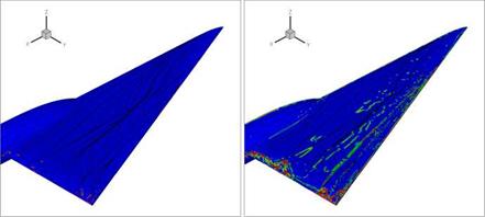
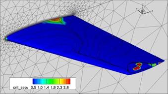
Fig. 28 VFE-2, coarse grid, WJ2D model — critical points of separation and reattachment (red) (left) and qualitative separation structure visualisation (right)

Field of Application and Its Limits

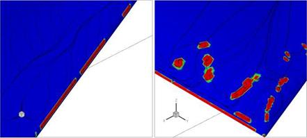
Fig. 29 VFE-2, coarse grid, WJ2D model — a detailed illustration of the critical points of separation with the output variable crit_sep (red), the separation of the primary vortex on the leading edge (left) and same small vortices near the trailing edge (right).

Field of Application and Its Limits

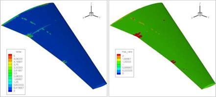
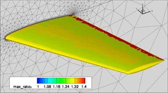
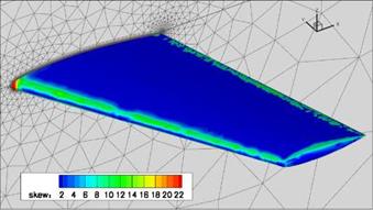
Fig. 30 SFB-401, coarse grid, SAE model — illustration of the average grid inclination in the boundary layer in degree (left) and the maximum expansion ratio in the boundary layer (right)

wall distance in the range of y+ = [0.01,5], the grid inclination in the range of a = [0, +/ — 70] and the wall normal grid expansion in the range of r = [1.1,2.0]. In the estimations the average inclination angle and the maximum expansion ratio were assumed as constant and only the greatest possible error is given.

Industrial Application

To test the sensors on industrial test-cases the generic 3D delta wing VFE-2 and the 3D airfoil SFB^01 were simulated. The delta wing VFE-2 shows a separa­tion of a primary vortex on the leading edge with a reattchment on the wing, which leads to a separation and reattchment of a secondary vortex. On the left-hand side in the figure 28 the critical points of separation and reattachment are shown (red), which presents the separation of the primary vortex on the leading edge and the vor­tex near the trailing edge very well. The separation of the secondary vortex and the

Industrial Application Industrial Application

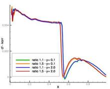
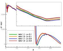
Fig. 26 RAE 2822 case9 — the errors in the expansion ratio and the wall distance leads to differences in the prediction of the friction coefficient Cf, in case of the mixed error both errors annul each other

Fig. 27 RAE 2822 case9 — the friction coefficient cf Corr corrected by the error function implemented in TAU, the differences are clearly reduced reattachment of the primary and secondary vortex are not identified. Both are identi­fiable in the output of the qualitative variable sep for separation structure visualisa­tion in the same figure on the right-hand side. In figure 29 a detailed illustration of the critical points of separation with the output variable crit_sep are shown, with the separation of the primary vortex on the leading edge (left) and same small vor­tices near the trailing edge (right). The sensors for the inclination and the expansion ratio are applied on the test-case SFB-401. The results are shown in figure 30.

Applicability on Mixed Errors

To test the applicability of the sensors on mixed errors the test-case RAE 2822 was examined. In figure 26 the friction coefficients of the test-cases with the separated and combined errors are compared with the reference test-case. The errors in the expansion ratio and the wall distance leads to differences in the prediction of the

Applicability on Mixed Errors

Fig. 24 ONERA M6, coarse grid — characteristic points of flow separation and reattachment and vortex separation at the airfoil tip

Applicability on Mixed Errors

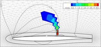
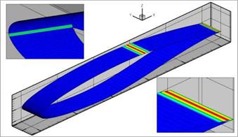
Fig. 25 RAE 2822 case9 — identification of the area of a compression shock

friction coefficient Cf and in case of the mixed error both errors annul each other. With correction of the predicted friction by the error function implemented in TAU the differences are clearly reduced (fig. 27).

Boundary Layer

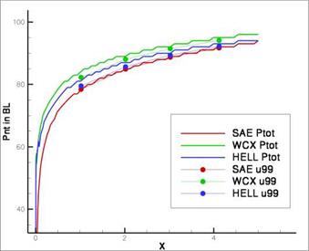
As graphical output the number of grid points in the boundary layer and the bound­ary layer thickness 3 in m is given in the flow solver output.

Separation

As graphical output the surface elements including characteristic points of separa­tion and reattachment plus both surface and volume elements with stagnation areas are marked in the flow solver output. Additionally the flow solver can give number of marked elements as a textual feedback.

Shock

As graphical output the volume elements including the characteristics of a shock are marked in the flow solver output. Additionally the flow solver can give a tendential prognosis of the position of the shock depending on the choice of the turbulence model. This is based on the investigations with the 2D RAE test-case.

Boundary Layer

Fig. 22 Flat plate — comparison of the number of points in the boundary layer detected by the sensor and with the boundary layer defined by 99% of the farfield velocity U99 with the SAE, Wilcox k-m and Hellsten EARSM model

Boundary Layer

Fig. 23 RAE 2822 case9 — characteristic points of flow separation and reattachment after the shock and near the trailing esge and the stagnation point

Uncertainty Sensors

For visualization of the uncertainties the areas of a shock based on Mach number and pressure gradients, areas of stagnation and surface elements including 1st or­der critical points of separation and reattachment are marked in the output routines.

Uncertainty Sensors

Fig. 21 ONERA M6, very coarse grid — expansion ratio of the grid in the boundary layer

Additionally the number of marked elements, the points in the boundary layers and the boundary layer thickness were written out as further information.

Grid Inclination

The graphical surface output of the inclination of the grid is given as a average deviation from the wall normal vector in degree (fig. 17 & 18). Additionally the differences in the friction Cf to the results of the ideal reference grid were written out as an expected error in % (cfn • 100%).

Grid Inclination

Fig. 17 RAE 2822 case9 — inclination of the grid in the boundary layer in degree (left), error in Cf caused by the inclination in the boundary layer in % (right)

Grid Inclination

Wall Distance y+

Grid Inclination Grid Inclination

y+ is a standard surface output value of the flow solver TAU. With that the im­plemented sensors can calculate the estimated error caused by the wall distance (fig. 19). This represents the predicted difference to the results of a simulation with the reference grid and a very small y+ in %.

Fig. 19 RAE 2822 case9 — wall distance (left), error in cf caused by the wall distance in % (right)

Application of the Sensors

For the usage of the sensors in the standard parameter files some variables were added to activate the best practice guidelines, the visual output and warnings.

4.1 Error Sensors

Application of the SensorsAfter activation of the best practice output and declaration of the directory contain­ing the configuration files of the best practice guidelines, the functionality of the individual sensors can be switched on and off. The configuration files are necessary to estimate the errors in the friction coefficients depending on the used model. These files contain a parameterized form of the error function as a polynomial 3rd order
(p(x) = a0 + a1x + a2x2 + a3x3) and the range of validity of this function. The func­tion represents the influence of the error on the friction coefficient and is computed by Cf normalized by the friction in the reference grid Cfn = cf /cf, ref. In addition for all errors a warning is given about the resulting influence on the skin friction component of the integral force coefficients. For this the drag coefficient was cor­rected by the resulting error in the friction and integrated along the wall surface. The computed and the corrected coefficients are compared and the result is written as a feedback in the flow solver output in %.

The error output and prediction are available for the turbulence models listed in Section 4.

Shocks

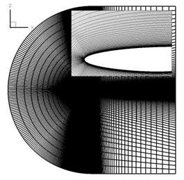
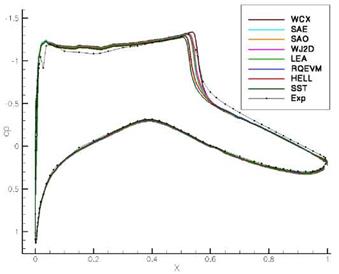
The correct prediction of flows with high pressure gradients, especially at shocks, also varies with the choice of the turbulence model, both in position and intensity. This again leads to changing values of lift and drag. For the investigation of this influence the 2D test-case RAE 2822 case 9 (Re = 6.5e6, Ma = 0.73) with a = 2.8 angle of attack and a shock at 55% chord length was applied. The grid is fully struc­tured and consists of 200,000 grid points (fig. 13). It has an orthogonal wall resolu­tion and a highly resolved boundary layer to exclude influences of errors. To achieve a more universal forecast for the computation of the shock position variations of the angle of attack (a = [1.0deg, 3.2deg]), the Mach number (Ma = [0.72…0.76]) and Reynolds number (Re = [6.0 • 106…107]) were investigated.

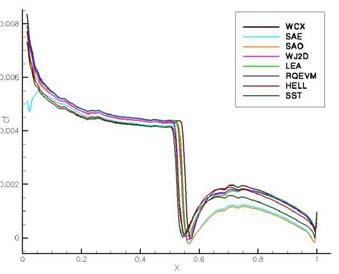
The variation of the turbulence models leads to visible variations in the shock position and the level of the cp and Cf coefficients (fig. 14 & 15). In comparison to the experiment the lift coefficient differs up to 4.6% and the drag coefficient up to 8.9% (e. g. Hellsten). The range between the models is +/ – 3.33% in the lift,

Shocks

Fig. 13 Grid of the RAE 2822 test-case with 200,000 grid points

Shocks

Fig. 14 RAE 2822 case9 — pressure coefficient Cp in comparision with the eight different turbulence models and the experiment

+/ — 7.55% in the drag coefficient and +/ — 2.86% in the shock position around the average of the results. There are obvious dependencies on the choice of the turbulence model and the shock position correlates very well with the lift coefficient. The results have shown that in the most investigated test-cases the prediction of

Shocks

Fig. 15 RAE 2822 case9 — friction coefficient Cf in comparision with the eight different turbulence models

Table 2 RAE2822 case9 – lift and drag coefficient, shock position compared to experimental results

CL

diff. in %

CD

diff. in %

shock xj c

diff. in %

Experiment

HELL

0.8030

0.7998

-0.40

1.6800E-02

1.6410E-02

-2.32

0.5500

0.5500

0.00

LEA

0.8224

2.42

1.7720E-02

5.48

0.5610

2.00

RQEVM

0.8055

0.31

1.7130E-02

1.96

0.5540

0.73

SAE

0.8244

2.67

1.6240E-02

-3.33

0.5640

2.55

SAO

0.8225

2.43

1.7110E-02

1.85

0.5630

2.36

SST

0.7858

-2.14

1.5730E-02

-6.37

0.5430

-1.27

WCX

0.8400

4.61

1.8300E-02

8.93

0.5750

4.55

WJ2D

0.8284

3.16

1.7770E-02

5.77

0.5650

2.73

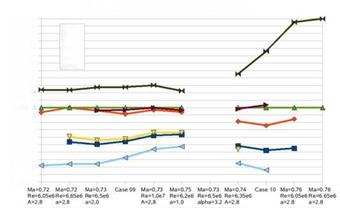
the shock position correlates with the turbulence model (left-hand side, fig. 16). In cases where another uncertainty exists, for example a separation bubble, (right-hand side, fig. 16, divergent progress) there is no exact forecast possible for the model dependency. Because of the unchanged order of the models a user feedback that shows only tendency is still possible.

1,060E+0 1.055E+0 1.050E+0 1.045E+0 1.040E+0 1.035E+0 1.030E+0 1.025E+0 1.020E+0 1.015E+0 1.010E+0 1.005E+0 1.000E+0 9.950E-1 9.900E-1 9.850E-1 9.800E-1 9.750E-1 9.700E-1 9.650E-1 9.600E-1 9.550E-1 9.500E-1

Подпись:Подпись: В HELL ф LEA VRQEVM ^SAE ► SAO <g|SST ►4 wcxFig. 16 RAE 2822 case9 — Position of the compression shock normalized by the position of the SAE model with variations of Mach number, Reynolds number and angle of attack

Implementation of the Shock Sensor

To detect a compression shock all grid elements were scanned of characteristic phys­ical values and marked if they exceed a given limit. These values are high pressure gradients in flow direction and a Mach numbers near 1. By projection of the nor­malized pressure gradients on the velocity a factor for the relative pressure increase was achieved and should come to 30%. The deviation of the Mach number from 1 should be less than 5%. These limits can be adjusted in the TAU solver butrepresent in all investigated test-cases very good indicators for a shock. The marked areas are available as an output value in the TAU routines.