Category Management and Minimisation of Uncertainties and Errors in Numerical Aerodynamics

The semi-infinite reformulation aims at optimizing the average objective function but maintaining the feasibility with respect to the constraints everywhere. Thus, it aims at an average optimal and always feasible robust solution. The ideal formula­tion is of the form

min f(y, p, s(Z))dP (Z) (23)

y, p

n

s. t. c(y, p,s(Z))= 0, yz є n (24)

h(y, p,s(Z)) > 0, yZ є П (25)

This definition of robustness can also be found in Ref.[21] and in Ref.[30] . Semi­infinite optimization problems have been treated directly so far only for rather small and weakly nonlinear problems, e. g. Ref.[10]. For the numerical treatment of com­plicated design tasks, one has to approximate the integral in the objective (23). Con­sidering scalar-valued uncertainties, we assume a truncated normal distribution, that means in the multivariate case з ~ шпН(у, С) • Ід, R C with expected value

1, if x є R

vector v, Covariance C and indicator function 1R(x) = .

0, if хЄ R

The integral in (23) can be efficiently evaluated by a Gaussian quadrature for small stochastic dimensions, where the quadrature points {з;}^=1 are the roots of a polynomial belonging to a class of orthogonal polynomials. Due to the exponen­tial growth of the effort with increasing dimension, the full tensor product Gaussian quadrature rule should be replaced in the higher dimensional case by Smolyak type
algorithms which use a recursive contribution of lower-order tensor products to es­timate the integral We will discuss this method in the next section. Therefore, we can reformulate problem (23-25) in an approximate fashion in the form of a multiple set-point problem for the set-points {s^N^:

N

min У f(yt, p, si)Oi (26)

Уі, Р =1

s. t. c(yi, p,Si) = 0, Vie{1,…,N} (27)

h(yi, p, Si) > 0, Vi e{1,…,N}. (28)

where <oi denote the quadrature weights. We will investigate this formulation later on.

The usual single setpoint aerodynamic shape optimization problem can be described in the following rather abstract form

min f(y, p) (14)

y, p

s. t. c(y, p) = 0 (15)

h(y, p) > 0 (16)

We think of equation (15) as the discretized outer flow equation around, e. g., an airfoil described by geometry parameter p e R”p. The vector y is the state vec­tor (velocities, pressure,…) of the flow model (15) and we assume that (15) can be solved uniquely for y for all reasonable geometries p. The objective in (14) f : (y, p) ^ f (y, p) e К typically is the drag to be minimized. The restriction (16) typically denotes lift or pitching moment requirements. To make the discussion here simpler, we assume a scalar valued restriction, i. e., h(y, p) e R. The generalization of the discussions below to more than one restriction is straight forward. In con­trast to previous papers on robust aerodynamic optimization, we treat the angle of attack as an fixed parameter which is not adjusted to reach the required lift (cf. e. g. Ref.[29], Ref.[21], Ref.[36] ).

The general deterministic problem formulation (14-16) is influenced by stochastic perturbations. We assume that there are uncertain disturbances involved in the form of real-valued random variables з : Q ^ R (or random vectors) associated with a probability measure P with Lebesgue density ф : R ^ R+ such that the expected value of з can be written as

E (s) = s(Z)dP (Z) = хф(х)<іх

Q R

and the expected value of any function g : R ^ R is written as

E(g(s)) = / g(s(Z))dP(Z) = / g(xMx)dx

Q R

The dependence can arise in all aspects, i. e., a naive stochastic variant might be rewritten as

min f (y, p, s) (17)

y, p

s. t. c(y, p, s)= 0 (18)

h(y, p, s) > 0 (19)

This formulation still treats the uncertain parameter as an additional fixed para­meter. The optimal solution should be stable with respect to stochastic variations in s. The literature can be classified in the following ideal classes: min-max formula­tion, semi-infinite formulation and chance constraints.

1.2 Min-Max Formulations

The min-max formulation aims at the worst-case scenario.

The min-max formulation is obviously independent of the stochastic measure P and thus needs only the realizations of the random variable з as input. If the probab­ility density function of the uncertain parameter is not available, this approach could potentially be an attractive strategy. Otherwise, this formulaion will ignore problem specific information, if it is at hand and will lead to overly conservative designs. We do not treat this formulation furthermore in this paper.

The Karhunen-Loeve-Expansion, also known as Proper Orthogonal Decomposition, represents the random field as a infinite linear combination of orthogonal functions chosen as the eigenfunctions of the covariance function [23], [31]. The Karhunen – Loeve-Expansion of the Gaussian random field у is given as:

V(-T C) = Vo (x) + X vbz, (x) Yj(Z) (7)

i=1

= fjV^iZi(x)Yi(Z) xer, Ze£2 (8)

i=1

where A1 > A2 > … > Xi > … > 0 and zi are the eigenvalues and eigenfunctions of the covariance function Cov which is symmetric and positive definite by definition. The deterministic eigenfunctions zi are obtained from the spectral decomposition of the covariance function via solution of

Г Cov (x, y) Zi (y) dy = XiZi (x). (9)

Having the eigenpairs, the uncorrelated Gaussian random variables Yi in equation (8) can be expressed as

Yi(C) = Ay [ V(x, C)zi(x)dx j = 1,2,… (10)

h Jr

with zero mean and unit variance, i. e. E (Yi) = 0 and E (YiYj) = Sij for j = 1,2,…

[5] . In the special case of a Gaussian random field, uncorrelated random variables are independent as well, which is an important property we will need later on for the sparse grid.

Truncating now the Karhunen-Loeve-Expansion after a finite number of terms, we obtain the approximation of the random field у

d

Wd(x, C) = JJ^zi(x)Yi(Q хеГХеП. (11)

i=1

The corresponding covariance function is given by

d

Covd (x, y) = ^hiZi (x) Zi (y). (12)

i=1

In [15], it is shown that the eigenfunction basis {zi} is optimal in the sense that the mean square error resulting from the truncation after the dth term is minimized.

The following approximation error representation is then obtained by Mercer’s theorem [34]

So, yd may provide a suitable approximation of у, if the eigenvalues decay suffi­ciently fast and d is large enough [5]. If one assumes a Gaussian covariance func­tion (cf. (5)), the eigenvalues will exponentially decay towards zero. The proof of this behaviour of the eigenvalues can be found e. g. [11]. This paper also provides a fast algorithm based on a kernel independent fast multipole method to compute the Karhunen-Loeve approximation. Another approach to solve the large eigenvalue problem arising from the Karhunen-Loeve-Expansion can be found in [25]. They in­troduce a Krylov subspace method with a sparse matrix approximation using sparse hierarchical matrix techniques to solve it.

The geometrical uncertainties also depend on the geometry itself, so they are modeled as a Gaussian random field

у: Г x Q ^ R, (3)

defined on a probability space (Q, Y,P) and on the shape of the airfoil Г. In each point x of the shape Г, the uncertainty is described by a normally distributed random variable y(x, ■) : Q ^ R. Additionally, the second order statistics, the mean value and the covariance function, are given to fully describe the random field. According to the scalar-valued uncertainties, the mean value of the random field у is equal to 0, since we expect no perturbations and the squared exponential covariance function describes the interaction between the random variables on the shape:

E(y(x, Z)) = У0 (x) = 0 Ух є Г (4)

Cov(x, y) = b2 • exp Ух, у Є Г (5)

The parameter l determines how quickly the covariance falls off and b controls the magnitude of the bumps. A squared exponential covariance function is chosen, since the resulting perturbed geometry is smooth due to the smoothness of the random field.

Then, a perturbed geometry is given as

v (x, Z) = x + y(x, Z) ■ n (x) Ух є Г, Z є Q (6)

where n is the unit vector in x normal to the profile Г. As we need to compute statistics of the flow depending on the uncertainty in our optimization algorithm, we have to approximate and discretize the probability spaces. In the next chapter, we will introduce the Karhunen-Loeve-Expansion which provides an approximation of the random field у for the numerical evaluation of such statistics and efficient discretization techniques of the probability space.

Since we want to avoid a parametrization of the uncertainties which would lead to a reduction of the space of realizations, we choose a stochastic approach in or­der to include the uncertainties in the optimization problem. Furthermore, this ap­proach allows to adapt the robust optimization to new information of the uncertain parameter, e. g. if new measurements are available, so that a general framework of robust aerodynamic design can be developed.

The proper treatment of the uncertainties within a numerical context is a very im­portant challenge, since the simulation and also optimization under uncertainties is a fast growing field of research. Again, we distinguish between the uncertainties with respect to the flight conditions, the scalar-valued uncertainties, and the geometrical uncertainties, the function-valued uncertainties.

1.1.1 Scalar-Valued Uncertainties

The scalar-valued uncertainties, e. g. the Mach number, are modeled as real-valued, continuous random variables

у: Q ^ R, (1)

defined on a given probability space (Q, Y,P). They are characterized by a given probability density function

Фtruncated : R ^ R+ • (2)

We assume (mainly due to lack of statistical data) a truncated normal distribution of the perturbations ensuring that the realizations lie in between the given bounds. Furthermore, the mean value of the random variable corresponds with the value of the deterministic model. These assumptions are widely used in order to describe uncertainties in CFD (cf. [32]). Nevertheless, the model need to be adapted to meas­urements, if available.

Aleatory uncertainties arises because of natural, unpredictable variations of the boundary conditions. Additional knowledge cannot reduce aleatory uncertainties, but it may be useful in getting a better characterization of the variability. In order to formulate the robust design optimization problem, we analyze the boundary condi­tions and input parameters identifying the uncertainties which cannot be avoided at all before constructing an aircraft [39].

In the following, we distinguish two types of uncertainties: uncertainties with respect to the flight conditions and geometrical uncertainties.

The main characteristics of the macroscopic flight conditions are angle of incid­ence, the velocity (Mach number) of the plane, the density of air and the Reynolds number. The uncertainty of these parameters mostly results from atmospheric turbu­lences which can occur during a flight. Gusts causes changes of the velocity in the range of ±10™. Measurements of the changes in the angle of attack and the density are not published so far, so they are assumed to be less than 10% of the setpoint. The variations of the Reynolds number will only effect the simulation, if the Reynolds number is in the range of 12 – 15 • 106, that means this uncertain parameter has not to be taken into account in our testcases.

On the other hand, we consider the shape itself as an uncertainty source. The real shape may vary from the planned shape due to manufacturing tolerances, temporary factors like icing e. g. or fatigue of material. Since there are so many factors hav­ing effects on the shape, this uncertainty has to be considered in the optimization problem in order to produce a design which is robust to small perturbations of the shape itself. In the literature, there can be found only a few papers on this topic investigating the influence of variations of the profile (cf. [17], [32]).

Volker Schulz and Claudia Schillings

Abstract. Recently, optimization has become an integral part of the aerodynamic design process chain. However, because of uncertainties with respect to the flight conditions and geometry uncertainties, a design optimized by a traditional design optimization method seeking only optimality may not achieve its expected perform­ance. Robust optimization deals with optimal designs, which are robust with re­spect to small (or even large) perturbations of the optimization setpoint conditions. That means, the optimal designs computed should still be good designs, even if the input parameters for the optimization problem formulation are changed by a non­negligible amount. Thus even more experimental or numerical effort can be saved. In this paper, we aim at an improvement of existing simulation and optimization technology, developed in the German collaborative effort MEGADESIGN[3] [4], so that numerical uncertainties are identified, quantized and included in the overall optim­ization procedure, thus making robust design in this sense possible. We introduce two robust formulations of the aerodynamic optimization problem which we numer­ically compare in a 2d testcase under uncertain flight conditions. Beside the scalar valued uncertainties we consider the shape itself as an uncertainty source and apply a Karhunen-Loeve expansion to approximate the infinite-dimensional probability space. To overcome the curse of dimensionality an adaptively refined sparse grid is used in order to compute statistics of the solution.

1 Introduction

Uncertainties pose problems for the reliability of numerical computations and their results in all technical contexts one can think of. They have the potential to render worthless even highly sophisticated numerical approaches, since their conclusions do not realize in practice due to unavoidable variations in problem data. The proper treatment of these uncertainties within a numerical context is a very important chal­lenge. This paper is devoted to the enhancement of highly efficient optimal design techniques developed in the framework of MEGADESIGN by a robustness com­ponent, which tries to make the optimal design generated a still good design, if the setting of a specific design point is varied.

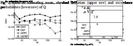
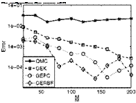
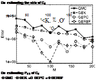
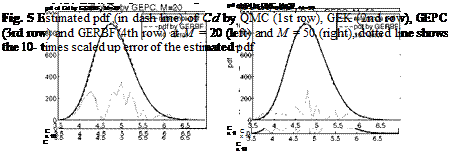
The results of the efficiency comparison are shown in Figure 2 to 5. Figure 2 and 3 show the errors of the four methods in estimating the target statistics of Q and Cd. It is observed there that the three gradient-employing surrogate methods, GEK, GEPC and GERBF are more efficient than the QMC method since the former three reduce their errors faster with an increasing cost measure M. Figure 4 and 5 depict the estimated pdf of Q and Cd obtained by the four methods, comparing with the refer­ence pdf. There we see that for the same computational cost, the surrogate methods yield much more accurate pdf’s. This is consistent with their relative performance in estimating the statistics.

Fig. 3 Error in estimating mean, standard deviation (upper row) and exceedance probabilities (lower row) of Cd

One of the reasons for the relatively better performance of the surrogate methods is that they utilize more information with the same computational cost M, i. e. they use (1 +сІ)Ц – conditions (SRQ samples and gradients) while a direct integration method like QMC uses M conditions (SRQ samples only). This advantage is due to the cheaper cost of obtaining gradients by an adjoint solver in the case that the number of SRQ’s is smaller than the number of variables d, and is expected to increase with an increasing number of variables, d.

Although it seems that GEK and GERBF perform better than the other surrogate methods in estimating statistics of Q and Cd respectively, it may not be appropriate to base a general conclusion on that. In Figure 4 and 5 we see the three surrogate methods have similar accuracy in their estimated pdf of Q and Cd.

The efficiency of GEK or GERBF is sensitive to the choice of the covariance model or the radial basis function and also to the value of the internal paramet­ers, and excelling configurations of them are problem – and data-dependent. In this work, different techniques are used for the optimization of the internal parameters, i. e., maximum likelihood optimization for GEK and leave-one-out error minimiz­ation for GERBF. This may also influence their relative efficiency, possibly differ­ently in the Ci and Cd cases. Due to the complex nature of comparative efficiency of

surrogate methods with different configurations and internal optimization tech­niques and different target SRQ, here we do not try to draw a conclusion on this issue.

In the estimation of the statistics of Q we see GEPC is not always reducing its error with an increasing M. This might be ascribed to the fact that the number of polynomial chaos (PC) terms is not truncated according to the order of PC, but to

an arbitrary number which is half of the number of available conditions. A set of PC terms that is “incomplete” for a particular order might not lead to more accurate ap­proximations than a set with less number of terms but “complete” for a lower order. Nevertheless, GEPC has a favored property that we have no burden of choosing the best-fitting configuration for it.

4 Summary

Gradient-employing surrogate methods have an advantage in handling aerodynamic uncertainty quantification (UQ) problems in the cases that an adjoint solver is used and the number of system response quantities (SRQ) is smaller than the number of variables so that the gradients of SRQ can be obtained at a reduced cost. These methods construct surrogates of the CFD model so that the statistics of an uncertain SRQ can be integrated on the surrogates models.

For investigating the efficiency of the different UQ methods we set up a test case where the geometry of an RAE2822 airfoil is perturbed by a Gaussian random field which is parameterized by 10 independent variables. Three surrogate meth­ods, gradient-enhanced radial basis functions, gradient-enhanced point-collocation polynomial chaos and gradient-enhanced Kriging, together with a direct integration method, quasi-Monte Carlo (QMC) quadrature, are applied to the test case and com­pared in their efficiency in estimating some statistics and probability distribution of the uncertain lift and drag coefficients. The results show that with the same com­putational effort the gradient-employing surrogate methods achieve better accuracy than the QMC does.

According to Wiener [22], f (|) can be approximated by a truncated polynomial chaos expansion (PCE)

f(l) = І Wl) (1)

i=0

where Щ is Hermite polynomial chaos (PC) to which a detailed description can be found in, e. g. [18]. The total number of terms is K = (p + d)l/(pldl) with p the order of PC.

To determine the coefficients ci we use a point-collocation method similar to the one used in [15], the difference being that we utilize gradient information. In this gradient-enhanced point-collocation polynomial chaos (GEPC) method the c = {c0, Ci, •••, cK}T is determined by solving the following system,

denote the sample points. The K is chosen to be half of the number of available “con­ditions”, N(1 + d), for the best performance according to [15]. This over-determined system is solved by a Least Squares method.

For this UQ job we first establish a GEPC surrogate model of f (|) based on QMC samples of the CFD model, and compute the mean and the variance of f (|) directly from the coefficients,

Д = co, o2 = Z(ct)2 ■ E[V2(S)] (2)

i=1

The exceedance probabilities and pdf are integrated by a large number (105) of QMC samples on the surrogate model.

Kriging [9] approximates f (|) by a weighted linear combination of samples, i. e.

N

f (I) = r(I) + T w (S®)f (S®)

i=1

where f (%l’i)) are N samples of the SRQ. у and wi are determined by minimizing the variance of the error e = f — f with the assumptions that the expectation of e is zero and that f (|) honors a spatial correlation model. We use direct gradient – enhanced Kriging (GEK) [8] that incorporates gradient information as secondary samples by an extended spatial correlation model that accommodates gradients. We implement GEK using the Surrogate-Modeling for Aero-Data Toolbox (SMART) [13] developed at DLR, opting for ordinary Kriging and a correlation model of spline type which is considered the most efficient in similar situations in [17]. The internal parameters of the correlation model are fine-tuned to fit the sampled data by a maximum likelihood estimation [24].

For this UQ job we first establish a GEK surrogate model of f (|) based on QMC samples of the CFD model, and integrate for the target statistics and pdf by a large number (105) of QMC samples on the surrogate model.