Category Management and Minimisation of Uncertainties and Errors in Numerical Aerodynamics

Quasi-Monte Carlo Quadrature

Quasi-Monte Carlo (QMC) quadrature [7] samples at a low discrepancy set of points generated by deterministic number-theoretic formulas. The “discrepancy” here is a measurement of how much the distribution of this set of points deviates from the underlying pdf. A low discrepancy set of points achieves a higher degree of uniformity with respect to a given pdf than a pseudo-random set of points does. So QMC is usually much more efficient than a Monte Carlo quadrature. The error bound of QMC is of order O(N-1 (logN)d) in which d is the number of variables. In many cases this is quite a loose upper bound of the error, i. e. QMC often performs better than that.

A variety of low discrepancy point sets exist, e. g. Van der Corput, Halton, Sobol, Hammersley and Niederreiter point set. The last one is used in this work as it is considered the most efficient when d is large [19]. The point set is generated by the program from [4]. The statistics of the SRQ are directly computed from the samples.

3.1 Gradient-Enhanced Radial Basis Functions

The radial basis function (RBF) method [6] approximates an unknown function by a weighted linear combination of radial basis functions each being radially symmetric about a center. An RBF approximation takes the form

N

f(I) = Xwiфг(||| -1®||)

i=1

where фі are radial basis functions, || • || denotes the Euclidean norm, and are the N sample points each taken as the center of a radial basis function. Making f (|) interpolate the N samples leads to N linear equations. The coefficients wi are determined by solving this linear system.

Denoting the Euclidean distance from the center as r, popular types of ф(г) include Vr2 + a2 (multiquadric), 1 /s/r1 + a2 (inverse multiquadric), exp(-a2r2) (Gaussian) and r2 ln(ar) (thin plate spline), in which a is a parameter to be fine-tuned for a particular set of samples. Gradient-employing versions of RBF were proposed in [11, 20] where first-order derivatives of the SRQ are exploited and second-order derivatives of RBF are involved in the system.

In this work we propose a different gradient-employing RBF method that in­volves only the first-order derivative of RBF, termed gradient-enhanced RBF (GERBF). To accommodate the gradient informations of the SRQ, this method in­troduces additional RBF that are centered at non-sampled points, i. e. an GERBF approximation is

f(I) = X Wi Фі(ііі – I{i>l), with N < K < N(1 + d)

i=1

The I(i’> with i < N are sampled points, those with i > N are non-sampled points which can be chosen randomly as long as none of them duplicates the sampled ones. The coefficients w = {w0, w1, • • •, wK}T are determined by solving the following system,

Фw = f

in which

-ф^))

Ф2(||1))

… Фк(||1)) –

7(I|1))

ф(!^)

ф1(1)(І|1))

Ф2(^))

ф21)(||1))

… Фк (IlN))

… фРц^)

g

• • • S’

Ф^^)

ф21)(|^))

… Ф^Ц^)

, f=

f (1)(I|N))

фРИ^)

ф2Рі«)

… Ф^ЦШ)

f МЦЫ)

ФРц^)

Ф^ЦМ)

… 4d)aiN))_

f (d)(sm)_

with фР = дФі/d^j, = df/d^j. We chose. K = ^(1 +d) in this work, which results in an over-determined system that is solved by a Least Squares method.

A numerical comparison of the accuracy of the aforementioned four types of RBF in approximating this CFD model f (|) was made by the author. The result favors the inverse multiquadric RBF which is therefore used in this work for the comparison with other UQ methods. The internal parameter a is fine-tuned by a leave-one-out error minimizing procedure as in [3].

For this UQ job we first establish a GERBF surrogate model of f (|) based on QMC samples of the CFD model, and integrate for the target statistics and pdf by a large number (105) of QMC samples on the surrogate model.

Methods

Four methods are applied to the test case. They include three surrogate methods, i. e. gradient-enhanced radial basis functions (GERBF), gradient-enhanced Kriging (GEK) and gradient-enhanced point-collocation polynomial chaos (GEPC), and one direct integration method, i. e. quasi-Monte Carlo (QMC) quadrature. An introduc­tion of them is made in this section.

Since the gradients of the SRQ with respect to all the ten variables are computed by an adjoint solver at an additional cost of approximately one evaluation of the CFD model, to account for this additional cost we introduce the term elapsed time – penalized sample number M by making M = 2N for the three gradient-employing methods and M = N for QMC, with N the number of evaluations of the CFD model. Compared to the cost of evaluating the CFD model the computational overhead of constructing surrogates is negligible, so in the efficiency comparison we use M as the measure of computational cost.

In the aspect of design of experiment, the study in [23] shows surrogate models based on samples with relatively high degree of uniformity (using Latin Hyper-cube sampling) are more accurate than those based on samples of lower degree of uni­formity (using plain Monte-Carlo sampling). For all the four methods in this work we adopt the QMC sampling scheme [7] because it achieves even higher degree of sample uniformity than Latin Hyper-cube sampling.

We use the DLR-TAU code [10] to solve the CFD model. The geometry per­turbation is implemented by using a mesh deformation tool based on radial basis functions incorporated in the DLR-TAU code as described in [14].

Test Case

The test case we use in this work is a CFD model of the inviscid flow around a 2-dimensional RAE2822 airfoil at a Mach number of 0.73 and an angle of attack of

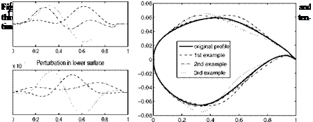
1.0 degrees. The source of uncertainty is the randomly perturbed airfoil geometry, i. e., the lower and upper surfaces of the airfoil’s 2D section (as shown by the solid line in the right part of Figure 1) are each assumed to be subject to a Gaussian random perturbation in the direction normal to the surface. Let pl and pu denotes the original lower and upper surface respectively, the perturbed surfaces are

Pi = pi + n • Є (x)

Pu = Pu + П • Єи(Х)

with x e [0,1]. n is the local normal vector of the surface, Є(х) is a zero-mean Gaussian variable with standard deviations a(x), i. e.

Єї(х),Єи(x) ~N(0,a(x))

in which

a(x)= 0.01 • Zmax • x( 1 – x) • 0(2,2)/1.5

with Zmax the maximum half-thickness of the airfoil, and в the Beta function. This setting makes the o(x) have its maximum (one percent of Zmax )at x = 0.5 and being zero at the two ends of the airfoil.

It is assumed that the random deformation is spatially correlated by a Gaussian type correlation function, i. e.

COv[e,(Xl),e,(x2)} = (7 (.n) (7 (-Г9 ) exp

= C(xb x2)

with I = 0.2. The same also applies to Єu(x).

For the purpose of numerical computation, the correlated random fields Єї (x) and Єи^) need to be represented in terms of uncorrelated random variables. This is furnished by Karhunen-Loeve expansions (KLE) [1], e. g. for Єї,

0i(x) = X у/%$Фі(х)

i=1

where are independent standard Gaussian variables. Xi and Фі (x) are the eigenval­ues and the eigenfunctions of C(xi, x2), i. e., the solutions of the following integral equation,

C(xbХ2)Фі(хі)йхі = Х1Ф1(Х2) Vі = 1,2,…

For practical problems the KLE needs to be truncated so that only a relatively small number of terms is kept, e. g. an approximation with к terms:

ві(х) « ^л/Хі^Фі(х)

i=1

By taking к = 5, 9i (x) is parameterized by 5 independent standard Gaussian vari­ables. Applying the same approximation to 9u(x),

2k

і=к+1

we express the randomly perturbed airfoil surface as a function of10 such variables. This KLE representation is optimal in the sense that it retains the original geometric variance to the maximum degree compared to any other linear-form representation with the same number of variables [1]. Figure 1 shows three examples of random perturbation in the upper and lower surface together with the corresponding per­turbed RAE2822 airfoil geometry.

Test Case

In this test case, the CFD model takes the input variables | = {|1; •••, £10} and yields the lift and drag coefficients, Ct and Cd, of the randomly perturbed airfoil. Hereafter, the model is denoted as f (|) in this paper. We compare the efficiency of the candidate methods in estimating some target statistics, i. e. the means (д jid), the standard deviations (at, ad) of Ct and Cd, and the exceedance probabilities Pf, j =

Pro{Q < p – j ■ ot} and Pd, j = Pro{Cd > Pd + j ■ Od} with j = 2,3. The accuracy of the statistics is judged by comparing with reference statistics obtained by a QMC integration with a large sample number (N = 2 x 10⁵).

Efficient Quantification of Aerodynamic Uncertainties Using Gradient-Employing Surrogate Methods

Dishi Liu

Abstract. Uncertainty quantification (UQ) in aerodynamic simulations is hindered by the high computational cost of CFD models. With gradient information obtained efficiently by using an adjoint solver, gradient-employing surrogate methods are promising in speeding up the UQ process. To investigate the efficiency of UQ meth­ods we apply gradient-enhanced radial basis functions, gradient-enhanced point – collocation polynomial chaos, gradient-enhanced Kriging and quasi-Monte Carlo (QMC) quadrature to a test case where the geometry of an RAE2822 airfoil is per­turbed by a Gaussian random field parameterized by 10 independent variables. The four methods are compared in their efficiency in estimating some statistics and the probability distribution of the uncertain lift and drag coefficients. The results show that with the same computational effort the gradient-employing surrogate methods achieve better accuracy than the QMC does.

1 Introduction

In aerodynamic simulations it is beneficial to consider uncertainties in the inputs, the formulation and the numerical error of the CFD model. In this work our concern is confined to the uncertainties in the model’s input and probabilistic approaches for uncertainty quantification (UQ) for CFD models. The uncertainties in the input propagates to the system response quantities (SRQ) through the model. Minor un­certainties can have an amplified impact in some instances and lead to occurrences of rare catastrophic events. Quantifying the uncertainties associated with the SRQ enhances the reliability of the simulations and enables robust design optimization. Most often this UQ process is done in a probabilistic framework in which the input

Dishi Liu

German Aerospace Center (DLR), Institute fur Aerodynamik und Stromungstechnik, Lilienthalplatz 7, 38108 Braunschweig, Germany e-mail: dishi. liu@dlr. de

B. Eisfeld et al. (Eds.): Management & Minimisation of Uncert. & Errors, NNFM 122, pp. 283-296. DOI: 10.1007/978-3-642-36185-2_12 © Springer-Verlag Berlin Heidelberg 2013

uncertainties are represented by random variables, and the consequent uncertainties in the SRQ are quantified by determining its probability distribution or statistical moments.

However, uncertainties in the input, especially those spatially or temporally dis­tributed, like geometric uncertainties, often generate a large number of variables. The “curse of dimensionality” prohibits the use of tensor-product quadratures. In [16] and [21] sparse grid quadratures were employed in aerodynamic UQ problems due to uncertain airfoil geometry. Nevertheless, if the number of variables is lar­ger than 10 even sparse grid methods suffer limitations in applicability [17]. The high computational cost of CFD models also makes the traditional sampling meth­ods such as Monte-Carlo and its variance-reduced variants (e. g. Latin Hypercube method) not efficient due to their slower error convergence rate.

Surrogate methods are gaining more attention in UQ as they provide approxim­ations of the CFD model which are much cheaper to evaluate while maintaining a reasonable accuracy so that the UQ can be performed on the basis of a large number of samples evaluated on the surrogate model. E. g. [12] shows a Kriging surrogate method better than plain Monte Carlo and Latin Hypercube methods in estimating the mean value of a bivariate Rosenbrock function. A comparative study of surrog­ate methods that are not employing gradients [23] shows Kriging is more accurate than radial basis functions and multivariate polynomial in approximating some 10- variate test functions.
Gradient-employing also give an edge to surrogate methods if the gradients are obtained at a relatively lower cost than that of the SRQ, which is the case when an adjoint CFD solver [5] is used and the number of SRQ is less than the number of variables. It should be noted that the gradient information cannot be effectively utilized by the UQ methods based on direct sampling of the CFD model. A naive augmentation of samples by finite difference brings no benefit because the augment­ing samples are not statistically independent of the original ones.

Different sampling schemes are adopted by surrogate methods, majorly of two groups: “on-grid” sampling and scattered sampling. The former is used in some methods based on polynomial approximations, e. g. stochastic collocation methods

[2] , and affected by the “curse of dimensionality” if the number of variables is large. The latter is more robust since it admits an arbitrary number of samples and arbitrary sample sites. This flexibility not only makes it tolerate sample failures (due to, e. g. poor convergence, as often observed in CFD models), but also makes an incorpor­ation of pre-existing or additional samples possible and enables run-time adaptive sampling.

In this work we apply three gradient-employing surrogate methods, i. e. gradient – enhanced radial basis functions (GERBF), gradient-enhanced point-collocation polynomial chaos (GEPC) and gradient-enhanced Kriging (GEK) [13], and for the purpose of comparison, also the quasi-Monte Carlo quadrature, to a UQ test case where an RAE2822 airfoil is subject to random geometric perturbations, and we compare their efficiency in estimating some statistics and probability distribution of the resulting uncertain lift and drag coefficients. The number of CFD model evaluations is kept small (< 200) in this numerical comparison to make it relev­ant to large-scale industrial applications.

Numerics

We demonstrate the influence of uncertainties in the angle of attack, the Mach num­ber and the airfoil geometry on the solution (the pressure, density, lift, drag, lift and absolute skin friction coefficients). As an example we consider two-dimensional RAE-2822 airfoil. The deterministic solver is the TAU code with the k-w turbulence model. To quantify uncertainties we used the collocation method computed in nodes of sparse Gauss-Hermite grid. The Hermite polynomials are of order P = {1,2, 4} with M random variables (see Eq. 10).

The last column in Tables 3 on the left and on the right shows the measure of uncertainty c/mean. It shows that 7.1% and 0.4% of uncertainties in a and in Ma correspondingly result in 4.4% and 16.3% (Table 3, on the right) of uncertainties in the lift CL and drag CD. For the comparison of different sparse grids see [13, 15].

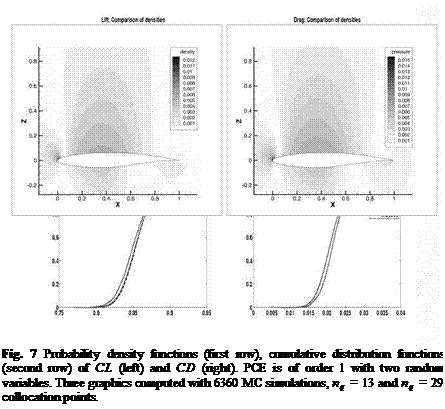
In Fig. 7 we compare the cumulative distribution and density functions for the lift and drag coefficients, obtained via PCE and via 6300 Monte Carlo simulations. The response surface is PCE of order 1. There are 106 MC evaluations of the response surface. We see three very similar graphics. Thus, one can make the conclusion that the sparse Gauss-Hermite grid with a small number of points, e. g. nq = 13, produces similar to MC results.

In Fig. 8 we compare the mean values computed by collocation and Monte Carlo methods for the Case 1. The collocation points are 281 nodes of two-dimensional

Подпись: mean st. dev. <T <T/mean a 2.8 0.2 0.071 Ma 0.73 0.0026 0.004 Подпись: mean st. dev. <T <T/mean CL 0.85 0.0373 0.044 CD 0.0187 0.00305 0.163

Table 3 Uncertainties in the input parameters (a(6, 02) and Ma(6, 62)) and in the solution (CL and CD). PCE of order 1 and sparse Gauss-Hermite grid with 137 points.

Numerics

Fig. 8 (left) ІІРМС “PSGhII and (rfght) 11 PMC “ PSGH II – PSGH was computed from the sparse Gauss Hermite grid with 281 nodes. PsgH ^ (0.65,1.2), p$GH ^ (0-7,1.3). Case 1.

sparse Gauss Hermite grid. One can see that the difference is very small compared to the corresponding physical values PsgH and PSGH.

Numerics

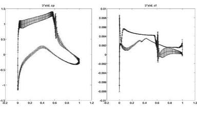
Fig. 9 3o error bars in each point of the RAE-2822 airfoil surface for the pressure coefficient cp (left) and friction coefficient cf (right).

The graphics in Fig. 9 demonstrate 3 a error bars, a the standard deviation, for the pressure cp and absolute skin friction cf coefficients in each surface point of the RAE-2822 airfoil. The data are obtained from 645 realisation of the solution. One can see that the largest uncertainty occurs at the shock (x « 0.6). A possible explanation is that the shock position is expected to change slightly with varying parameters a and Ma.

In Table 4 one can see relative errors of the rank-& approximations (in the Frobenius norm). Five solution matrices contain pressure, density, turbulence kin­etic energy (tke), turbulence omega (to) and eddy viscosity (ev) in the whole com­putational domain with 260000 dofs. Additionally, one can also see much smaller memory requirement (dense matrix format costs 1.25GB). The column 7 shows the computing time required for the SVD-update (the Algorithm described in Sec­tion 5.1) and the the column 8 time required for the full SVD of the global matrix Є r260000x600 correspondingly. A possible explanation for the large computing time for the full SVD is the lack of memory and expensive swapping of data.

Table 4 Relative errors and computational requirements of rank-k approximations of the solution matrices Є r260000x600. Memory required for the storage of each matrix in the dense matrix format is 1.25 GB.

rank k

pressure

density

tke

to

ev

time, sec update

time, sec full SYD

memory

MB

10

1.9e-2

1.9e-2

4.0e-3

1.4e-3

1.4e-3

107

1537

21

20

1.4e-2

1.3e-2

5.9e-3

З. Зе-4

4.1e-4

150

2084

42

50

5.3e-3

5.1e-3

1.5e-4

9.1e-5

7.7e-5

228

8236

104

Table 5 Rank-k approximation errors of the variance of pressure and of the variance of dens­ity in Case 9

rank к

5

30

max* var(p)(.x) – var(p)k(x)

5.3e-3

1.6e-4

max* | var (p) (x) – var (pk) (x)

3.5e-3

8.8e-5

In Table 5 we provide the rank k = {5,30} approximation errors (in the max­imum norm) of the variance of the pressure and of the density (compare with Fig. 5). The variances var(p)k(x) and var(pk)(x) were computed from the matrix W є R65568x1521 as described in Section 5.

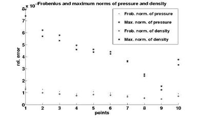
Further, we consider Case 1 (a = 1.93 and Ma = 0.676, no shock). Fig. 10 shows relative errors (for the Case 1) in the Frobenius and the maximum norms for pressure and density computed in 10 points of a two-dimensional sparse Gauss-Hermite grid. These relative errors compare the solution which we obtain after 10000 TAU itera­tions without any start value with the solution which we obtain after only 2000 TAU iterations with start values taken from the response surface (multivariate Hermite polynomials with M = 2 variables and of order P = 2). One can see that the errors are very small (of order 10~3), i. e. the response surface produces a good approxim­ation. We note that 10 chosen points are lying in a small neighbourhood of the point a = 1.93 andMa = 0.676.

Numerics

Fig. 10 Relative errors (Case 1) in the Frobenius and the maximum norms for the pressure and density

Bayesian Update of the Uncertain Airfoil Geometry

We assume that the airfoil geometry contains random deformations (e. g. dents). A possible reason, for example, can be the influence of external forces. First our task is to parametrize all such deformations for all given airfoils. We offer to use random fields к(х, со), where со is a vector of random parameters (see Section 2.2). The problem is that the probability density function of о is unknown. We assume it a priori as Gaussian. If we could measure all given airfoils (from different airplains) then we could build a good parametrization model, but everything we can do is to measure airfoils only in a few points. This is our knowledge. The question now is how to incorporate this knowledge to our parametrization model? We can do this by using the Bayesian update. The Algorithm is described in [21, 20].

Bayesian Update of the Uncertain Airfoil Geometry Bayesian Update of the Uncertain Airfoil Geometry

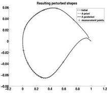
In Fig. 6 (left) you may see:

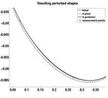
Fig. 6 (left) The truth airfoil (is in reality unknown), a priori (is our initial assumption) and a posteriori (the measurements are taken into account) airfoils. (right) Detailed RAE-2822 airfoil picture in interval [0.05, 0.35].

• The initial airfoil (dashed line). Is in real life, as a whole, unknown. One can measure it only in a few points.

• A priori realization (dash-dot line). One realization computed from the a priori model without any knowledge (without measurements). Usually does not coin­cide with the truth. Can be far away from the truth.

• A posteriori realization (solid line) is computed via the Bayesian update (see details of the Algorithm in [21, 20]) from the a posteriory model which takes into account the real data measured in the 8 measurement points (8 stars). Since large deformations are not allowed, all three curves are very similar. The detailed picture (in interval [0.05, 0.35]) is shown in Fig. 6 (right). One can see that the solid line (a posteriori model) is much closer to the measurement point (denoted by stars) than to the dash-dot line (a priori model).

Data Compression

A large number of stochastic realisations of random fields requires a large amount of memory and powerful computational resources. To decrease memory requirements and computing time we offer to use a low-rank approximation for all realisations of the solution [13]. This low-rank approximation allows us an effective postprocessing (computation of the mean value, variance, exceedance probability) with drastically reduced memory requirements (see Table 4). For each new realisation only the cor­responding low-rank update will be computed (see, e. g. [1]). This can be practical when, e. g. the results of many thousands Monte Carlo simulations should be com­puted and stored. Let v; є Rn, i = 1..Z, be the solution vector (already centred), where Z is a number of stochastic realisations of the solution. Let us build from all these vectors the matrix W = (vi,…, vZ) є RnxZ and consider the factorisation

W = ABT, where A є Rnxk and B є RZxk. (15)

We say that matrix W is a rank-k matrix if the representation in Eq. 15 is given. We denote the class of all rank-k matrices for which factors A and BT in Eq. 15 exist by R(k, n, Z).If W є R(k, n, Z) we say that W has a low-rank representation. The first aim is to compute a rank-k approximation Wk of W, such that

||W – Wk|| < e, k < min{n, Z}.

The second aim is to compute an update for the approximation Wk with a linear complexity for every new coming vector vZ+1. Below in Section 5.1 we present the algorithm which performs this.

To get the reduced singular value decomposition we omit all singular values, which are smaller than a given level e or, alternative variant, we leave a fixed number of largest singular values. After truncation we speak about reduced singular value decomposition (denoted by rSVD) Wk = UkZkVkT, where Uk є Rnxk contains the first k columns of U, Vk є RZxk contains the first k columns of V and Zk є Rkxk contains the k-biggest singular values of Z.

The computation of such basic statistics as the mean value, the variance, the ex­ceedance probability can be done with a linear complexity. The following examples illustrate computation of the mean value and the variance.

Let us take A := UkZk and BT := VT є RkxZ. Denote the j-th row of matrix A by aj є Rk and the i-th column of matrix BT by Ь; є Rk. It is evident, that if W is given explicitly, one can compute the mean value and the variance just keeping in memory 2 vectors – the mean (variance) and the current value. Below we show how to compute the mean and the variance if only A and B are given.

1. One can compute the mean solution v є R" as follows

1 z 1 z –

v= – XAb<=Ab. (Д6)

Z i=1 Z i=1

rank к

5

20

max* p (x) — pк (.r)

1.7e-6

4.2e-10

maxj 1 var(p) (x) – var (p )* (x)

6.7e-5

2.3e-8

Table 2 Rank-k approximation errors of the mean and of the variance of density in Case 1.

The computational complexity is O(k(Z + n)), in contrast to O(nZ)) for usual dense data format. As a demonstration we compute the mean.

2. One can compute the variance of the solution var(v) є Rn by the computing the covariance matrix and taking its diagonal. First, one computes the centred matrix

WC:=W —vlLr, where v = W • 1L/Z, and 11 = (1,…, 1)г є Rz. (17)

Computing Wc costs O(k2(n + Z)) (addition and truncation of rank-k matrices). By definition, the covariance matrix is C = . The reduced singular

Подпись: C Data Compression Data Compression Подпись: (18)

value decomposition of Wc is (Wc)k = UkZkVl, Uk є Rnxk, Ek є Rkxk and Vk є RZxk can be computed via the QR algorithm [5, 13]. Now, the covariance matrix can be written like

The variance of the solution vector (i. e. the diagonal of the covariance matrix C can be computed with the complexity O(k2(Z + n)).

Table 2 demonstrates the rank-5 and rank-20 approximations of the mean and of the variance of density. One can see that both rank-k approximation errors are very small, much smaller than e. g. the discretisation error or Monte Carlo error (by com­puting the mean value).

Lemma 0.1. Let ||W —W*||2 < є, апсіщ be a rank-k approximation of the mean її. Піепа)\й-щ\ <ф., b) j| Wc — (W с) л-11 < є, r)||C-C,|| <^e2.

Proof: Since її = 11 and її* = ^W*1L, then

] ] P

|u-u*.||2 = — ||(W-W*)U||2 <-||(W-W*)||2-||1L||2 < -7=

Ns Ns N

Let I є RNs xNs be the identity matrix, then

1 T

||Wc-(Wc)*||2< ||W-W*||2.||I – — – І-11г||2<є, and

Ns

Подпись: CC

*lb < ^jllWcWf – (Wc)*(Wc)[ |b

Подпись: Ns 1Ns 1

2.1 Concatenation of Two Low-Rank Matrices

Let A and B such that Wk = ABT be given. Suppose also that matrix W Є Rnxm contains new m solution vectors. For a small m, computing the factors C Є Rnxk and D Є Rmxk such that W « CDT is not expensive. Now our purpose is to compute with a linear complexity the rank-k approximation of Wnew := [WW’ ] Є Rnx (Z+m). To do this, we build two concatenated matrices Anew := [AC] Є Rnx2k and Bnew = blockdiag[BT DT] Є R2kx(Z+m). Note that the difficulty now is that matrices Anew and Bnew have rank 2k. The rank k approximation of the new matrix Wnew is done with a linear complexity O((n + Z)k2 + k3) (for details see [13]).

Update of the Low-Rank Response Surface via Computing the Residual

In real-world applications, the deterministic solver is very complicated and it is dif­ficult or even impossible to change it, but one can often print out the norm of the residual. Assume that we already approximated the unknown solution by a response surface. Our response surface is approximation via multivariate Hermite polynomi­als like in Eq. 14, where coefficients are computed like in Eq. 13 with quadrature points 9i, i = 1..nq. The following algorithm updates the given response surface. Algorithm: (Update of the response surface)

1. Take the next point 9nq+1 and evaluate the response surface Eq. 14 in this point. Let u(x, 9nq+i) be the obtained predicted solution.

2. Compute the norm of the residual ||r|| of the deterministic problem (e. g. evaluate one iteration). If ||r|| is small then there is no need to solve the expensive de­terministic problem in 9nq+i, otherwise (if ||r|| is large) solve the deterministic problem and recompute A, Br and cp in Eq. 12.

3. Go to item (1).

In the best case we never solve the deterministic problem again. In the worst case we must solve the deterministic problem for each 9nq+i, i = 1,2,… To test this al­gorithm we computed the solution in Case 1 with 10000 TAU iterations (is usual number of iterations). Then, first, we computed the solution with the response sur­face (as described above) and, second, corrected it with 1000 TAU iterations. Then we compared both solutions and observed only a very small difference. Thus, the response surface reduced the number of needed iterations from 10000 to 1000. We note that the solution in Case 1 is smooth and there is no shock.

We tested this Algorithm also in the Case 9 (solution with a shock) and it failed. We pre-computed the solution by two different response surfaces (of order P = 2 and P = 4). Both response surfaces failed to produce a good result. For instance, we observed not only one shock, but many smaller shocks. Then we observed an increasing range of e. g. pressure (range (—6;5) in contrast to (0.5,1.3)). It is similar when one tries to approximate a step function by a polynomial — the amplitude of oscillations grows up. Another negative effect which we observed during further iterating the solution, obtained from the response surface, was that the deterministic solver (TAU) produces “nan” after few iterations. A possible reason is that some important solution values, obtained from the response surface, are out of the physical range (e. g. negative density) and are non-realistic.

Thus, we can come to the conclusion that if the solution is smooth (e. g. as in Case 1) then response surface produces a good starting value. Otherwise, if the solution has a shock, the response surface produces a very poor approximation and further iterations do not help.

The computed solution u(x, 9nq+1) can be used to update the response surface, i. e. to recompute the matrices A, B and […c^…] and PCE coefficients (Eq. 13). Please note that this update works only in the case of the usage of embedded sparse grids or (Q)MC in Eq. 11.

Low-Rank Response Surface

To compute statistics of the random (uncertain) solution (error-bars, quantiles, cu­mulative density function, etc) accurate enough, one needs a large sample size. Monte Carlo simulations are expensive. To decrease the computational costs we compute a, so-called, response surface — (multivariate) polynomial (see Eq. 10). The idea [13] is to construct a good response surface from few samples and then
to use the residual for its improvement. A motivation for this idea comes from the fact that in many software packages for solving engineering and physical problems it is impossible or very difficult to change the code, but it is possible to access the residual. Later on the computed response surface is used for very fast generation of a large sample.

Let у(л;, в) be the solution ( or a functional of the solution). It can be pressure, density, velocity, lift, drag etc. v(x, в) can be approximated in a set of new independ­ent Gaussian random variables (truncated polynomial chaos expansions of Wiener [25])

(x, в(ю)) « X vp(x)Hp(e) = l-vp(x)-}l-Hp(e)-]T> (10)

Подпись: V/3(X> = -^J0Hp(e)v{x,e)¥{de) Low-Rank Response Surface Подпись: (11)

where coefficients vp (x) are computed as follows

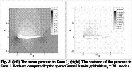
The PCE representation in Eq. 10 was used to compute the mean and the variance of the pressure (see Fig. 3) for the Case 1 (a = 1.93 and Ma = 0.676, no shock). PCE coefficients are computed by the sparse Gauss Hermite grid with nq = 281 nodes. Here the multidimensional integral over 0 is computed approximately, for example, on a sparse Gauss-Hermite grid [6, 2].

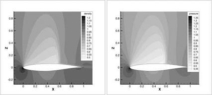
Fig. 4 demonstrates the mean of density and mean of pressure, computed again as in Eq. 10 for the Case 9 (a = 2.79 and Ma = 0.734, with shock).

Подпись: Fig. 3 (left) The mean pressure in Case 1; (right) The variance of the pressure in Case 1. Both are computed by the sparse Gauss Hermite grid with nq = 281 nodes.
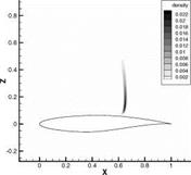
Fig. 5 demonstrates the variance of density and variance of pressure, computed via Monte Carlo methods for the Case 9. One can see the largest uncertainty in the shock position.

Low-Rank Response Surface

Low-Rank Response Surface

Fig. 4 (left) The mean density; (right) the mean pressure computed by PCE in the Case 9


Low-Rank Response SurfaceLow-Rank Response Surface

Fig. 5 (left) The variance of the density; (right) The variance of the pressure computed by MC in the Case 9.

Using the rank-k approximation of [v(x, Q1),.., v(x, 0nq)], obtain

V/зМ = – j^[(x,0i),…,(x, e„9)] ■ [Hp(ei)wi,…,Hp(6nq)w„g]T « АВГС|3, (12)

where A є Rnxk, B є Rnqxk, k min{n, nq} and

vector cp := – рї[Нр(ві)м? і, …,Нр(вПд)м? Пд]т. The matrix of all PCE coefficients will be

[…yp(x)…}= ABT[…ер…], в є Jm, p. (13)

Taking Eq. 10 and Eq. 13, obtain the final formula for the low-rank response surface

Discretisation Techniques

In the following, (Q, B, P) denotes a probability space, where Q is the set of ele­mentary events, B is the а-algebra of events and P is the probability measure. The symbol ю always specifies an elementary event ю e Q.

The random field k(x, ю) needs to be discretised both in the stochastic and in the spatial dimensions. One of the main tools here is the Karhunen-Loeve expansion (KLE) [16]. By definition, KLE of a random field к(х, ю) is the following series [16] „

к(х, со) = к(х) + X уД^ф((х)^(со), (6)

t=

where are uncorrelated random variables and k(x) is the mean value of

к(х, ю), Xt and фе are the eigenvalues and the eigenvectors of problem

Tфе = Хф фе e L2(G),е e N, (7)

and operator T is defined like follows

T : L2(G) ^ L2(G), (Tф)(х) := / cov*(x, у)фШу,

where covK is a given covariance function. Throwing away all unimportant terms in KLE, one obtains the truncated KLE, which is a sparse representation of the random field к(х, ю). Each random variable %e can be approximated in a set of new independent Gaussian random variables (polynomial chaos expansions (PCE) of Wiener [7, 25]), e. g.

&(ю)= E $Р)ни(в(®))’

^J

where 9(a) = (0i (a), 92(a),…), %(в) are coefficients, H are multivariate Hermite polynomials, в є J is a multiindex, J := {fifi = (p1,…,Pj,…), f5j є N0} is a multi-index set [18].

For the purpose of actual computation, truncate the polynomial chaos expansion after finitely many terms, e. g.

в є Jm, p := {в є J y(p) < M, P<P}, r(p) := max{j є Nв > 0}.

Since Hermite polynomials are orthogonal, the coefficients <^e) can be computed by projection

ф = ^Івщ{ете)те).

This multidimensional integral over 0 can be computed approximately, for ex­ample, on a sparse Gauss-Hermite grid with nq grid points

1 nq

* ji%Hp(8i)ZiWwi, (8)

where weights wi and points 9 і are defined from sparse Gauss-Hermite integration rule. After a finite element discretisation (see [10] for more details) the discrete eigenvalue problem (7) looks like

МСМф = Cij = covK(x, yj). (9)

Here the mass matrix M is stored in a usual data sparse format and the dense mat­rix C є Rnxn (requires O(n2) units of memory) is approximated in the sparse H – matrix format [10] (requires only O(n log n) units of memory) or in the Kronecker low-rank tensor format [9]. To compute m eigenvalues (m C n) and corresponding eigenvectors we apply the Lanczos eigenvalue solver [11, 22].