Category Management and Minimisation of Uncertainties and Errors in Numerical Aerodynamics

The MLS interpolation method was first applied to spatial coupling in aeroelasticity by Quaranta et al. [23]. It exclusively uses low-order polynomials

s(x) = mT (x) a (11)

to approximate the spatial deformation distribution u(X). At each CFD surface point X, a new set of Q polynomial coefficients a(X) is computed with a moving least – squares fit. The Ng closest support points Xn provide a compact support; their influ­ence relative to the CFD surface point is weighted with Wendland RBF (8). For each surface point X and its Ng support points inside the support radius g a functional

I(X, Xn)= 0(X, Xn) (mT (Xn) a(X) – Ux(X-n))2 dn(Xn) (12)

%

has to be minimised for the coefficients a(X). The discrete form of this functional is reduced to the normal equation through a variation of coefficients ga:

Herein, Ф(X, Xn) = E |0(X, Xn)} is the diagonal matrix of RBF weighting factors. Inserting the interpolation function (11) yields

ux(X)= mT(X) A-1B [ux(Xn)} . (14)

‘—— V—— ‘

=P(X)

The row matrix P(X) describes the projection between a single surface point X and the Ng support points inside the support radius. Other than in the GSB method, in the MLS method the projection matrix is built row by row for each surface point separately. The final projection matrix P is assembled from the M row matrices of all surface points. For each surface point a Q x Q-matrix A has to be set up and inverted. Its condition number and thus its invertability depends on the number of support points and their spatial arrangement. Practical experience has revealed that the regularisation of the linear systems of equations (13) by left multiplication of [m(Xn)] is highly detrimental to its condition number. A more accurate and robust numerical solution can be achieved if instead for each surface point the Ng overde­termined systems of equations

Ф(^, Xn) [m(Xn)]T [a*(Xn)] = Ф(^, Xn) (15)

are solved with QR decomposition, yielding Ng tuples of polynomial coefficients a*(Xn) for unit deflections u*x(Xn) at the individual support points. The final row entry to the projection matrix then is

P(x) = mT (X)[a*(xn)j. (16)

Because the interpolation function (11) has only local support, the projection mat­rix is sparse, greatly reducing memory requirements in comparison with the GSB method.

Investigations using configurations with multiple components revealed that even with these new projection methods explicitly based on interpolation schemes addi­tional interpolation in intersection regions between assemblies cannot be avoided. If the whole configuration is treated as a single assembly during the projection, the resulting deformed wetted surface is contiguous, but extremely distorted. (With the GSB method, its global polynomial term in the interpolation function can even result in an unfeasible propagation of deformations to assemblies not directly connected, e. g. from the main wing to the empennage.)

For the MLS scheme, an additional interpolation in intersection regions has been implemented that works in a similar fashion as the interpolation of the FIE method

(3) : For a surface point situated in an intersection region, as depicted on the left of Fig. 4, a row entry to the projection matrix Pk(X) is built for the element groups dir­ectly assigned. Further entries are built with the structures of each adjacent surface segment. The resulting K row entries are assigned normalised weights wk according to the surface point’s distance a to the intersection curve. Weighted averaging yields the final entry to the projection matrix for the given surface point:

KK

P(X) = £ wk(X, alimit) Pk(X) with £ wk(X, aUinit) = 1. (17)

k=1 k=1

This interpolation algorithm exploits the fact that the MLS method builds the pro­jection matrix one surface point at a time. In the GSB method, the projection matrix is created for all points simultaneously. To realise a comparable interpolation, for each assembly a projection matrix would have to be built which relates the points of its surface segment to all neighbouring structures. Only then the average can be taken with suitable weights assigned to the row entry of each surface point. Be­cause of the high memory requirements of just a single projection matrix result­ing from the GSB method, comparable interpolation has not been implemented in the ACM.

As alternatives to the existing FIE scheme, in the project MUNA, the spatial coup­ling schemes GSB and MLS were implemented in the ACM. They are closely related, as both cast the problem of projecting loads or deformations as an inter­polation problem: For a set of N points in space xn with dependent values f (xn) one seeks to find a functional approximation to f based on a suitable choice of interpol­ation functions. In this sense, the distribution of dependent values is the deformation u provided at the structural nodes. Its functional approximation is then evaluated at a second set of M points Xm, which are the points of the CFD surface mesh. The two projection methods differ in their choice of interpolation functions which dictates the solution process.

The GSB method was originally published by Beckert and Wendland [6]. The authors approximate the deformation on the whole domain with a global low-order polynomial with Q monomials. The monomial vectors are either

m = (1, x, y, z)T or m = (1, x, y, z, x2, y2, z2, xy, yz, zx)T. (6)

Superimposed are local contributions ф(х) that consist of radial basis functions (RBF). At a given coordinate, the interpolation function is

NS

s(x) = mT(x)в + X a(Xn) Ф(х, Xn). (7)

n=1

The coefficients a(Xn) of the local RBF contributions and the coefficient vectors в of the global polynomial are calculated simultaneously for all Ng support points with a weighted least-squares algorithm. The dependent values at the interpolation support points are reproduced exactly. The RBFs with compact support constructed by Wendland [30] serve as weighting functions. The C2-continuous Wendland-RBF with a support radius g is provided here as an example:

ф(х, x„) = (1 – x)+(4x+l) with x= ||x — x„ ||2 • (8)

The index + marks that the factor (1 – x)4 is set to zero for values of x > 1, whereby the compact support is realised. The functional approximation to the deformation distribution can be obtained from the linear system of equations

"[ф(х„ X,)] [mr (x0] ] ({a H = f {uX(xj ^ 1 1 < i ;< Ns (9)

L [m(Xj)] 0 J j в J = 0 }’ 1 — i ’ j – Ng ’ (9)

‘————– V————- ‘

=C

which has to be solved for each Cartesian displacement component X = x, y, z. (Here, scalar quantities that are combined to a vector are put in braces. Brackets denote that scalars or vectors that are assembled to form a matrix.) This process would have to be repeated in each coupling step; instead the inverse of the coeffi­cients matrix C is determined. The functional approximation can now be evaluated at the surface points, which yields the final projection matrix P:

In the GSB method the support radius g has to be the same all over the computa­tional domain, or else the interpolation scheme will not be consistent. In general, the number of support points Ng will differ from one CFD surface node to the next. The user has to define a minimum required number of support points and the projec­tion scheme searches the domain for the smallest radius g that contains this number. Because of the global contribution to the interpolation function the resulting pro­jection matrix is dense. Its definition here (and in the MLS method) differs from the definition in Eq. (2) in that here the deformations or forces are projected one spatial component X at a time. The GSB method is largely identical to the volume mesh deformation method presented by Barnewitz in this volume. The main differ­ence lies in the choice of weighting functions and the compact support of the local contributions to the interpolation function.

For structural models with a single straight beam axis, the FIE method is a logical extension of beam theory. The projection algorithm assures that during deformation sections through the wetted surface that were perpendicular to the beam axis in the undeformed configuration preserve their shape. If however a structure consists of several angled beam segments, possibly part of different assemblies such as a wing and fuselage, a straightforward application of the described algorithm can lead to a non-smooth or non-contiguous deformed wetted surface.

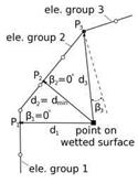
With configurations comprising more than one assembly, any projection between surface components and structural model parts not physically connected must be avoided. This is exemplified in Fig. 3 for a high-lift device. The structural elements closest to surface points along the trailing edge actually belong to the flap. Projec­tions based solely on shortest distance lead to a physically impossible transfer of loads and deformations over the flap gap. This is prevented by explicitly assigning structural elements to surface segments of the individual assemblies. In a prepar­atory step all collinear beam elements of each assembly are combined in element groups. Each assembly’s surface segment is given a unique identifier. In the ACM’s input data set, the element groups are then either assigned to surface segments or ex­cluded from the projection algorithm. In the current example, the flap track elements should be excluded because they have no wetted surface segments as counterparts for mapping.

However, the strict application of this explicit assigning can make the wetted surface come apart at intersections between assemblies: Due to their projection on

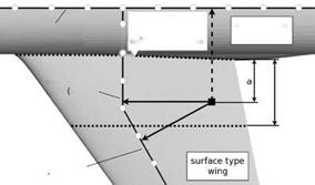
elements of different element groups, those neighbouring surface points which are part of different assemblies can experience incompatible deflections. The two sur­face segments necessarily contiguous in the undeformed configuration are no longer so after the deformation projection. The resulting defective mesh is not suitable any more for flow computations. This problem is resolved by means of an interpolation algorithm, which is exemplified by the wing-fuselage joint shown in the left image of Fig. 4. First, all seam curves between adjacent surface segments are detected. For a surface point belonging e. g. to the main wing, the projection is carried out onto the directly assigned element groups of the wing, giving a “direct” deflection uC^. Next, the projection is repeated for the element groups assigned to the neighbouring fuselage surface, which gives an “indirect” deflection u£pD. The weighted average of the two contributions is take

Alimit and dlimit are user-defined parameters which determine the extent of the in­terpolation region. The final surface point deflection is then interpolated from all considered projection results:

ucfd = X Wtot, i ucfd, i with Wtot, i

i

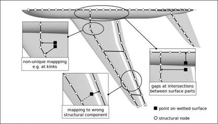
Fig. 4 left: Blending in the vicinity of intersections between surface segments of differ­ent assemblies, here at the wing-fuselage joint. right: Interpolation regions with non-unique mapping near kinks of the beam axis.

All interpolations have to be applied in the same manner also during the load pro­jection as otherwise the conservativity would be violated (cf. Eq. (2)).

The FIE projection method, also known as inverse isoparametric mapping, uses the shape functions of the FE structural model to interpolate loads and deformations between the points on the wetted surface and the nodes of the structural model. This results in an efficient algorithm which only requires the evaluation of algebraic expressions. The FIE method is briefly demonstrated here in conjunction with beam models. For a more elaborate description extended to structural models consisting of volume and shell elements the reader may refer to Reimer et al. [25].

The FIE method is based on purely geometrical considerations. In the first step, the closest structural element for a given point on the wetted surface is sought. In­side this element the projection point is determined. For a beam model this point

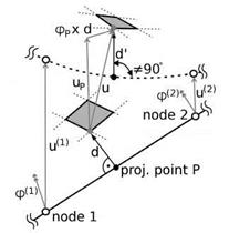
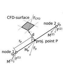
Fig. 2 Load and deformation projection with FIE on beam elements. left: Projection of aerodynamic forces from the wetted surface to the structure. right: Projection of deformations from the structure back to the wetted surface.

generally creates a perpendicular connection between surface point and beam axis, as depicted on the left of Fig. 2. The aerodynamic surface load Fcfd is shifted along the distance vector d to the projection point P and an equivalent offset mo­ment MP = d x FcFD is introduced. With the shape functions of the element and the natural coordinate of the projection point rP the force and the moment are divided among the element’s nodes. The closest elements and natural coordinates of the projection points are determined only once before the first coupling step and then reused. During the deformation projection shown on the right of Fig. 2 the corres­ponding steps are carried out in opposite order: The rotational deformation (pP and the translational deformation uP at the projection point are interpolated from the nodal values with the element shape functions. The deflection of the surface point consists of uP and a rotational contribution pP x d. Even if the projection point on the undeformed beam axis created a perpendicular connection between beam axis and surface point, due to shear this may not be the case in the deformed configura­tion, represented by the dashed line in Fig. 2.

The methodology applied for structural models comprising shell or volume ele­ments, which have two-dimensional projection surfaces, is the same in principle. A more involved algorithm is required to find the projection point on the closest element face. Interpolation in intersection regions has not been realised yet, so that with such structural models the FIE method in the ACM can be applied only to con­figurations with one assembly. The CVT method can be seen as a variant of the FIE method in which the length of the distance vector is no longer kept constant, but adapted according to the deformational change of the area of the projection face.

The analyses presented in the paper at hand concentrate on error sources in spa­tial coupling, and so the description of the projection methods shall be afforded a separate section here. To begin with, an overview of projection methods suitable for reduced structural models is given. The existing projection method based on Fi­nite Interpolation Elements (FIE) is explained. Then the newly-implemented Global Spline-Based (GSB) and Moving Least-Squares (MLS) methods are presented in detail.

In order to be valid from the physical point of view, any projection scheme has to be conservative with the following two criteria: First of all, the total force and moment vectors must be preserved during the projection. Secondly, during steady simulations the elastic strain energy of the structure must be identical to the work performed by the aerodynamic loads on the wetted surface, as implied by Eq. (2). During unsteady simulations also the instantaneous power exchanged over the coup­ling surface must be the same on both sides. From the flow solver and the volume mesh deformation code, further numerical requirements arise affecting the projec­tion of deformations from the structure back to the wetted surface: The resulting deformed surface mesh should be contiguous in particular at intersections between the surface meshes of distinct assemblies, for instance between fuselage and wing. The deformed surface mesh should be smooth in order to assure good convergence of the flow solution. One final demand is of a more practical nature: With reduced structural models, any projection scheme has to make some kind of assumption for the transfer of forces and deformations over the gap between wetted surface and structure. This assumption should not be far removed from the load paths actu­ally to be expected, i. e. some measure of locality should be preserved during the projection.

Initially, only one projection algorithm was available inside the ACM: The Fi­nite Interpolation Element (FIE) method [5, 8, 9, 25] is an uncomplicated method that uses the shape functions of the structural model to divide aerodynamic surface loads among the nodes of the closest structural element. During the first phase of MUNA, a number of alternative projection methods was reviewed for inclusion in the ACM. Many published methods are only adequate for configurations where the wetted surface and the surface of the structural model coincide up to the discret­isation error [10, 17, 22, 29]. On account of the requirements set forth for reduced

structural models such methods were excluded. Prospective methods included the Infinite-Plate Spline (IPS) method [14], the Constant-Volume-Tetrahedron (CVT) method [2, 13] and the inverse Boundary Element Method (BEM) [11]. These were extensively compared by Sadeghi et al. [27]. The GSB method [6] and the MLS method [23] constitute further alternatives suitable for reduced structural models.

With the IPS method, only the deflections normal to the wing plan form are in­terpolated from the structure to the wetted surface using splines as interpolation functions. This limits the method to (almost) planar configurations. With the CVT method, tetrahedra are spanned between the points on the wetted surface and the nodes of the closest structural element. Both the natural coordinates of the projec­tion point inside the element and the volume of the tetrahedron are kept constant for all deformation states, defining the projection. As will become evident further down, the CVT method can be regarded as an extension of the FIE method. The BEM method is the projection method which is most firmly footed on physical con­siderations instead of geometrical neighbourhood relations: The gap between wetted surface and structure is modelled as an elastic continuum, and the deformation of the structure is expressed in terms of surface deflections through the BEM. This relation then has to be inverted with the minimisation of the elastic strain energy of the continuum as an additional constraint. Of all methods presented so far this is the most demanding. Furthermore, it requires the connectivity of the wetted surface, which currently is not transmitted from the flow solver to the ACM. The GSB and MLS methods both determine a function approximation to the nodal displacement distribution and evaluate it at the surface points. The two methods differ primarily in their choice of interpolation functions. They do not interfere with the modular structure of the ACM, offer the required generality, are independent of the dimen­sionality of the structural model and involve only a moderate implementation effort. Also, there is a significant implementation overlap between them, for which reason both were selected for inclusion in the ACM.

For the volume mesh deformation of structured FLOWer meshes, the Multiblock Grid Deformation Tool (MUGRIDO) [8,16] was developed at LFM. This tool mod­els the block boundaries of the volume mesh and selected additional mesh lines as massless Timoshenko beams. The deflections of the surface nodes relative to the undeformed configuration are imposed as boundary conditions and the struc­tural problem is solved. Finally, the positions of the remaining mesh points inside of the blocks are calculated with transfinite interpolation. MUGRIDO is not suit­able for unstructured TAU meshes. TAU offers two mesh deformation algorithms;

best suited for aeroelastic simulations with complex configurations is the weighted volume spline interpolation algorithm [15]. A further description can be found in the paper by Barnewitz in this volume. Since this method does not require any informa­tion regarding the connectivity between volume mesh points, it is equally applicable to structured meshes.

For the computation of the structural deformation, the in-house structural solver “Finite Element Analysis for Aeroelasticity” (FEAFA) is employed. It is a Finite Element (FE) code based on a physically and geometrically linearised formulation, so it is limited to small strains and linear-elastic material behaviour. Over recent years, it has been expanded to offer a range of element types comparable to com­mercial CSD code packages which includes volume and shell elements, spring ele­ments, point masses and multi-freedom constraints. The mainstay for aeroelastic simulations is the multi-axial Timoshenko beam element [8, 9]. Its formulation al­lows for distinct cross-sectional positions of the centre of mass, the shear centre and the centre of bending. Thereby structural coupling between bending and torsional motion can be captured. The consideration of shear deformation in the Timoshenko formulations assures a physically-reasonable wave propagation through the struc­ture, which is important for unsteady simulations. With very few degrees of freedom and thus at low computational cost, such reduced structural models are capable of accurately rendering the elastic and inertial properties of slender structures such as transport aircraft wings. This is not only a significant advantage for unsteady sim­ulations, but also for steady design optimisation tasks, as has been demonstrated in the MEGADESIGN [20] project. During steady simulations, the structural deform­ation is either obtained by direct solution of the linear system of equations resulting from the FE discretisation or by superposition of pre-calculated modes.

To date, the ACM has been coupled with three Reynolds-Averaged Navier-Stokes (RANS) Finite-Volume flow solvers: FLOWer [18, 19], TAU (recent developments are highlighted in a number of papers in this volume) and QUADFLOW [3]. In this paper, results obtained with FLOWer and with TAU are presented. The development of both solvers was initiated and led by the DLR. Further enhancement of the struc­tured solver for multi-block topologies—FLOWer— may not be actively promoted anymore, but with that solver the greatest amount of experience has been gained in conjunction with the ACM, and the coupling can be regarded as well-validated against experiments. The effort to couple the ACM with the hybrid-unstructured solver TAU began during the previous project MEGADESIGN [20] and, for the steady branch, has been completed during MUNA. The interfaces of both flow solv­ers with the ACM provide the same functionality, but their implementation is quite different. FLOWer simply calls the ACM as a Fortran subroutine. The loads and load incidence points and the coordinates of the deformed wetted surface are exchanged via the subroutine parameter field. The communication between TAU and ACM used to be realised by files written on hard disk, but is now carried out completely in-memory. The solution is controlled through a script written in the object-oriented scripting language Python [26]. TAU and its components already have Python in­terfaces and are suitably wrapped during compilation. The ACM has to be provided as a shared object file. Specific Python interface classes contain the methods and attributes needed to perform the aeroelastic coupling. In each coupling step, the ACM’s Python interface reads the loads and load incidence points from TAU’s C data stream and passes them on to the ACM. In the reverse direction at the end of a coupling iteration, the interface receives the coordinates of the deformed wetted surface from the ACM and writes these to the data stream. All the while the interface has to ensure that the fields are passed on correctly between the individual software components written either in C, Fortran or Python.

For an investigation of the actual projection process it may not be relevant whether or not the loads on the wetted surface result from a flow simulation. In certain cases a user-defined load distribution may be imposed instead. This is pos­sible with the stand-alone version of the ACM. Obviously, conclusions drawn in this manner can only regard the projection algorithm as such and not the coupled solution process as a whole.

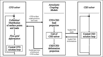
All algorithms for the simulation of fluid-structure interaction problems fall into one of two major categories: Monolithic algorithms solve the equations governing the flow field and those governing the structural deformation simultaneously as a single set of equations [7, 21]. Partitioned algorithms employ dedicated solvers for each field which are coupled via a suitable interface. The monolithic method en­sures that the mutually dependent solutions in each field are always on the same time level, which eliminates the issue of synchronising individual solvers for a con­servative solution. In practise, though, this method has one significant disadvantage, which has limited its acceptance: A monolithic coupled solver generally has to be developed completely from scratch, whereas with a partitioned approach one can employ pre-existing single-field solvers and benefit from the developments of spe­cialised research groups. Ideally, the necessary coupling interface should be suf­ficiently modular to allow the replacement of a single-field solver either with an updated version or with an entirely different implementation. The aeroelastic code package conceived at LFM/CATS, henceforth denoted as “Aeroelastic Coupling Module” (ACM) [9, 24, 25], is based on this rationale. The ACM allows the modu­lar coupling of arbitrary flow and structural solvers with only minor code changes. Both steady simulations with a staggered (Block-Gauss-Seidel) algorithm and un­steady simulations with weak and strong temporal coupling schemes are possible. Pursuant to the partitioned approach followed here, the ACM serves as the interface between the dedicated single-field solvers for the flow field and for the structural deformation, as is shown in Fig. 1. The ACM carries out the synchronisation of the solvers by initiating iteratively their respective calls.

Apart from the synchronisation of the single-field solvers, the ACM also per­forms the spatial coupling, i. e. the projection of loads from the wetted surface to the structure and in reverse direction the projection of the structural deformations to the wetted surface. The projection methods available are tailored to reduced struc­tural models. These are beneficial especially during unsteady simulations because of their smaller number of degrees of freedom and thus lower requirements of com­putational resources. With reduced structural models the geometries of the wetted surface and of the structural model coincide only in parts or not at all. This is es­pecially true for beam models which do not even share the same dimensionality as the wetted surface. Also with more detailed models like shell models, in many cases one does not want to represent the complete structure. When modelling a wing, of­ten only the wing box is taken into consideration. The high lift devices and other components which do not contribute significantly to the overall structural stiffness are disregarded. In both examples there are “gaps” between the wetted surface and the structural model which have to be bridged by the projection algorithm.

Because of these gaps between wetted surface and structure, forces have to be projected from the wetted surface to the structure instead of surface stresses. Latter do not possess an effective direction required in this case. As to increase the mod­ularity of the ACM, the aerodynamic surface forces are calculated already inside the flow solver and passed on to the ACM. They should be derived in a consistent manner from the discrete distribution of surface stresses [12]. The ACM receives a cloud of load incidence points with associated force vectors and returns a cloud of surface coordinates representing the deformed wetted surface. Thus, the ACM can be coupled with structured and unstructured flow solvers alike since it is independ­ent of the manner in which points are associated with surface cells. As a side note, the number of the load incidence points and their position in the undeformed wet­ted surface do not have to be identical with the surface points defining the wetted surface.

To summarise above statements, the aeroelastic coupling with the ACM com­prises three steps:

1. From the pressure and surface stress distribution on the wetted surface, discrete force vectors are determined by the flow solver.

2. These surface forces are projected from the wetted surface to the nodes of the structural model.

3. The structural deformations resulting from the projected load distribution are projected back onto the wetted surface.

Each of these steps may contribute to the total error of the coupled simulation scheme. The second and third ones are closely related, though: The projection of (generalised) forces from the wetted surface to the structure can conveniently be ex­pressed as a matrix-vector product with a force projection matrix Pf, and likewise the projection of (generalised) deformations can be expressed with a deformation projection matrix PU:

The conservativity of the projection method is assured if Pu = PTF, which can be shown via the principle of virtual work [12]:

SWcfD = FCfd ^UCFD SWcsD = FcSd ^UCSD

= FCFD PU ^UCSD = (PFFCFD)T ^uCSD (2)

= FCFD PF ^UCSD

Consequently, the same projection method has to be used during the projection of forces as during the projection of deformations.

A fourth step, external to the ACM, involves the deformation of the CFD volume mesh in order to accommodate the deformed wetted surface. Mesh deformation methods generally depend on the formulation of the flow solver employed, and their associated error sources are not investigated here.

Georg Wellmer, Lars Reimer, Horst Flister, Marek Behr, and Josef Ballmann

Abstract. In this paper, the realisation and testing of spatial coupling methods for aeroelastic simulations with partitioned algorithms is presented. The investigated methods for spatial coupling—the transfer of loads and deformations between the wetted surface and the structural model—are the method of Finite Interpolation Ele­ments and two other, newly-implemented interpolation methods. All three are suit­able for reduced structural models, and the geometries of the wetted surface and the structural model do not have to coincide. The aeroelastic simulation tool employed and the theoretical background of the spatial coupling schemes are outlined. Differ­ent measures for the quality of the spatial coupling are derived and applied to test cases of increasing complexity. The influence of user-defined coupling parameters on the deformation projection is assessed. Based on these results and on practical considerations, the available coupling methods are compared and conclusions are drawn regarding their applicability.

1 Introduction

The civilian aircraft industry faces the necessity to reduce aircraft fuel consumption while increasing flight safety levels and maintaining passenger comfort. Further­more, competition on the aircraft market forces manufacturers to accelerate design cycles and to reduce the costs of the actual development. This twofold pressure has brought about the widespread adoption of numerical prediction methods during all

Marek Behr • Georg Wellmer • Lars Reimer

Chair for Computational Analysis of Technical Systems (CATS), Center for Computational Engineering Science (CCES), RWTH Aachen University, SchinkelstraBe 2, 52062 Aachen e-mail: {wellmer, reimer, behr}@cats. rwth-aachen. de

Josef Ballmann

Lehr – und Forschungsgebiet fur Mechanik (LFM), RWTH Aachen University,

SchinkelstraBe 2, 52062 Aachen

e-mail: ballmann@lufmech. rwth-aachen. de

B. Eisfeld et al. (Eds.): Management & Minimisation ofUncert. & Errors, NNFM 122, pp. 181-218. DOI: 10.1007/978-3-642-36185-2_8 © Springer-Verlag Berlin Heidelberg 2013

stages of the design process. Computational Fluid Dynamics (CFD) for the numer­ical prediction of the flow field about aircraft configurations are of special interest to the industry. These methods have matured to a point where they are not merely complementing costly wind tunnel test campaigns, but actually partially supplanting them. Simultaneously, improvements in structural analysis methods such as Com­putational Structural Dynamics (CSD) and in material sciences have led to lighter aircraft frames with greater inherent elasticity. Aeroelastic coupling effects now def­initely have to be considered in the design process and thus also have to be captured by the numerical prediction methods, i. e. by Computational Aeroelasticity (CAE) solvers. A code package for the simulation of the interaction between aerodynamic, elastic and inertial forces has been developed at LFM/CATS over the last decade. Work was initiated at LFM within the framework of the Collaborative Research Centre 401 (SFB 401) [3, 28] and continued at CATS, in the course of the collabor­ative research project MUNA, amongst others.

In order for CAE to gain the same acceptance in the aerospace community as that already enjoyed by CFD, its solutions must prove to be trustworthy. Engin­eers require the numerical predictions design decisions are based on to have a de­pendable accuracy, which can be evaluated in two different manners: First of all, by comparison with experimental results the error incurred by the whole coupled algorithm can be estimated. It can then be used as a measure of confidence for nu­merical predictions regarding comparable configurations. Validation against steady and unsteady wind tunnel data has been carried out continuously at LFM/CATS, most recently in the project “High Reynolds Number Aero-Structural Dynam­ics” (HIRENASD) [4, 24]. This approach has the downside that without extensive parameter studies the cause of deviations—potentially each of the single-field

solvers or their mutual interaction—cannot be easily determined. Besides, it must not be forgotten that also measurements inevitably have an error. In the second ap­proach error sources are identified and examined individually, at least as far as such a separation is possible. Regarding aeroelastic coupling, it has to be demonstrated that associated sources of error do not significantly impair the accuracy of the over­all coupled solution. This method often is feasible for model test cases only, and the findings have to be scrutinised before being applied to real-world problems. Dur­ing the MUNA project both outlined investigation methods have been applied at LFM/CATS with regard to steady aeroelastic simulations and their associated error sources.

This paper will take the following outline: First the coupling methodology in general and the algorithm developed at LFM/CATS in particular are delineated, as well as the available spatial coupling methods. The potential error sources are defined and their influence is quantified for model problems. Next, the assessment is repeated for actual coupled flow simulations. Based on the results, the available methods for spatial coupling are compared and a set of recommendations is derived.