Category A PRACTICAL. APPROACH TO. ROBUSTNESS. ANALYSIS

THE LINEARIZED MODEL

THE LINEARIZED MODEL

The above model is linearized at a medium value r = 1 0 deg of the angle of attack. The following LTI model is obtained:

This model is essentially parameterized by the 4 stability derivatives MQ, Ms, Za and Zs – For the sake of simplicity, it was assumed that cos(a) « 1 in equation (2.7), so that Ma and Za correspond to the linearization of the nonlinear functions Cn(a,6,M) and Cm(a,6,M) with respect to a. On the other hand, Ms and Zs coincide with the quantities dn and dm in equation (2.9).

THE LINEARIZED MODEL

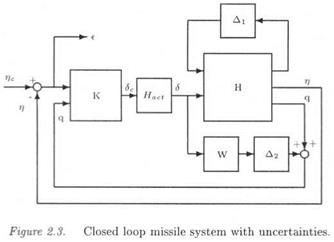
The issue in the following will be to analyze the local stability and performance properties of the closed loop missile in the presence of para­metric uncertainties in these 4 stability derivatives and in the face of neglected dynamics, namely a high frequency bending mode. To this aim, the parametrically uncertain missile model will be first transformed into a standard LFT structure Fu(H(s),Ai), where Ді gathers the un­certainties in the stability derivatives. On the other hand, the bending mode is represented by an additive model perturbation ДгЫ and its template 1/ W(5) is extracted from (Reichert, 1992; Balas and Packard, 1992). The uncertain closed loop missile is presented in Figure 2.3, where K(s) represents the missile autopilot. Note that the weights in the sta­bility derivatives are chosen as 5 %. In the context of Д» control, the frequency domain performance is defined through the sensitivity func­tion S, i. e. the transfer between the commanded acceleration r)c and the tracking error e = r)c — rj.

THE NONLINEAR MODEL

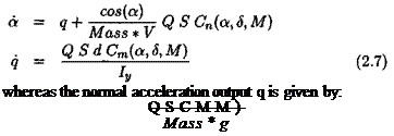
Подпись: whereas the normal acceleration output q is given by: QSCMM) Mass * g

A nonlinear longitudinal missile model is extracted from (Reichert, 1992). The control input is the tail deflection <5, while the outputs used by the autopilot are the acceleration and rate outputs [ту, q). The state vector is [ct, <?], where a is the angle of attack. The missile behavior can be described by the following nonlinear equations:

This model is essentially parameterized by the Mach number M (between 2 and 4). The dynamic pressure 0, the reference area S, the diameter d, the pitch moment of inertia Iy and the missile mass are indeed constant, while the missile velocity V is proportional to M. Cn and Cm depend on M, a and 8:

Cn(a,8,M) = ana3 + bnaa + c„(2 – M/3)a + dn8 Cm(a,8,M) = ama3 + bmaa + cTO(—7 + 8M/3)a + dmS (2.9)

See (Reichert, 1992) for numerical data. The main nonlinearities are the variation of Cn(a,8,M) and Cm(a, S,M) as a function of a, since these quantities are third order polynomials of a, whose range of variation is ± 20degrees. The actuator is finally a second order transfer function:

Подпись: Wact

Подпись: + 1
Подпись: +

Hact{s) = – Г2 ~~2fZTT~T (2.10)

with u>act = 1 5 0 rad/s and £act = 0.7.

A MISSILE PROBLEM

The nonlinear aerodynamic model is described in the first subsection, while the linearized model is presented in the second one. The #<*> autopilot is synthesized in the third subsection.

Glossary

a: angle of attack. q: pitch rotational rate.

6: actual tail deflection angle.

Sc: commanded tail deflection angle. rjc: commanded acceleration. rj: actual acceleration.

M: Mach number.

V: missile velocity.

Mass: missile mass.

Iy pitch moment of inertia.

Q: dynamic pressure.

S: reference area. d: missile diameter.

DESIGN OF A FLEXIBLE CONTROLLER

An observed state feedback controller is synthesized. On the one hand, the rigid closed loop poles are placed in the same way as in subsection 1.2. On the other hand, some of the flexible modes are moved into the left half plane in order to increase their damping ratio.

Following the previous subsection, the design model is built by adding the rigid and flexible models at the outputs. Actuators are then in­troduced at the aircraft inputs (see Figure 2.2). Second order transfer functions ————;— are finally added at the inputs, with —^ = 0.0 and

u>f = 15 rad/s. These filters increase the roll-off properties of the con­troller, and thus its robustness with respect to unmodeled flexible modes. Notice that the maximal frequency of the bending modes in the previous subsection is about 15 rad/s.

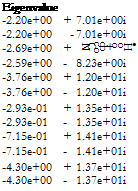
A state feedback controller is first synthesized for this design model. The actuators and filters poles are not to be moved. The four rigid closed loop poles are chosen as in subsection 1.2. The 6 closed loop flexible modes are chosen as:

Deunping

Freq. (rad/s)

З. ООе-ОІ

7.35е+00

3.00е-01

7.35e+00

3.00е-01

8.62е+00

З. ООе-ОІ

8.62е+00

З. ООе-01

1.25е+01

З. ООе-01

1.25е+01

2.16е-02

1.35е+01

2.16е-02

1.35е+01

5.07е-02

І.4ІЄ+01

5.07е-02

1.4ІЄ+01

З. ООе-01

1.43е+01

З. ООе-01

1.43е+01

Подпись: Eigenvalue -2.20e+00 + 7.01e+00i -2.20e+00 - 7.01e+00i -2.69e+00 + •H о о + ф со CN CD -2.59e+00 - 8.23е+00і -3.76e+00 + 1.20e+01i -3.76e+00 - 1.20e+01i -2.93e-01 + 1.35e+01i -2.93e-01 - 1.35e+01i -7.15e-01 + 1.41e+01i -7.15e-01 - 1.41e+01i -4.30e+00 + 1.37e+01i -4.30e+00 - 1.37e+01i

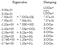
The damping ratios of the 4 critical flexible modes are increased up to 30 %. The two other flexible modes are left unchanged. Summarizing, the closed loop poles, corresponding to the state-feedback controller, are:

Подпись:Freq. (rad/s)

9.00e-01 У. rigid modes

9.50Є-01

9.90e-01

9.90e-01

7.35e+00 V, flexible modes

7.35e+00

8.62e+00

8.62e+00

1.25e+01

1.25e+01

-2.93e-01

+

1.35e+01i

2.166-02

1.356+01

-2.936-01

1.356+01І

2.166-02

1.35e+01

-7.156-01

+

1.4І6+01І

5.076-02

1.4І6+01

-7.156-01

1.4І6+01І

5.076-02

1.4І6+01

О

о

+

ф

о

со

1

+

1.376+0ІІ

З. ООе-01

1.436+01

-4.306+00

1.37e+01i

З. ООе-01

1.436+01

-1.056+01

+

1.076+01І

7.006-01

І. БОе+01

‘/. filter modes

-1.056+01

1.07e+01i

7.00в-01

1.506+01

1

»-»■

о

СП

ф

+

о

+

1.076+01І

7.00в-01

1.506+01

-1.056+01

1.076+01І

7.006-01

1.506+01

-1.046+01

l. OOe+OO

1.046+01

‘/, actuator modes

-І. Обв+01

l. OOe+OO

І. Обе+ОІ

-3.766+01

l. OOe+OO

3.766+01

-3.376+01

+

3.876+01і

б. ббе-01

Б. ІЗв+01

-3.376+01

3.876+Oli

6.566-01

5.136+01

An observer is now to be built. Since the states of the filters are available, the new design model is the same as the one for the state feedback, except that it does not include the filters. The observer gain places the closed loop poles roughly in the same way as the state feedback gain. When applying the observed state feedback controller to the complete aircraft model (which thus includes the rigid model, the flexible model and the actuators), the closed loop poles are classically the poles of the state – feedback controller and those of the observer.

. THE FLEXIBLE MODEL

A complete model of the aircraft is obtained by adding its rigid and flexible models at the outputs (see Figure 2.2). A real modal state – space representation of the flexible part is given in appendix A. The corresponding flexible modes are:

Eigenvalue

Damping

Freq. (rad/s)

-2.42Є-01

+

7.34e+00i

3.29Є-02

7.35Є+00

-2.42Є-01

7.34e+00i

3.29е-02

7.35е+00

-4.39e-01

+

8.бІе+ООі

5.09е-02

8.62е+00

-4.39e-01

8.бІе+ООі

5.09Є-02

8.62е+00

-З. ОЗе-01

+

1.25е+01і

2.42е-02

1.25е+01

-З. ОЗе-01

1.25е+01і

2.42е-02

1.25Є+01

-2.93Є-01

+

1.35е+01і

2.1бе-02

1.35Є+01

-2.93Є-01

1.35е+01і

2.16Є-02

1.35Є+01

-7.15e-01

+

1.4ІЄ+01І

5.07е-02

1.4ІЄ+01

-7.15е-01

1.4ІЄ+01І

5.07Є-02

1.4ІЄ+01

-2.24e-01

+

1.43е+01і

І. Ббе-02

1.43Є+01

-2.24Є-01

1.43е+01і

1.56е-02

1.43Є+01

In chapter 4, uncertainties in the natural frequencies of the bending modes above will be introduced in the aircraft model.

. DESIGN OF A RIGID CONTROL LAW

A static output feedback K assigns the closed loop eigenstructure, and a static feedforward H introduces the pilot demands in the closed loop, which is summarized in Figure 2.1.

Подпись: Eigenvalue Подпись: Damping Подпись: Freq. (rad/s)

The gain matrix K is synthesized with a classical modal approach with decoupling objectives. The poles of the open loop aerodynamic model (i. e. the rigid model without actuators) are:

Подпись:3.4ІЄ-03 – l. OOe+OO -5.Ole-02 + 6.74e-01i 7.4ІЄ-02 -5.0ІЄ-02 – 6.74e-01i 7.4ІЄ-02 -8.59Є-01 l. OOe+OO

The corresponding closed loop poles are chosen as:

Подпись: EigenvalueПодпись:

. DESIGN OF A RIGID CONTROL LAW

Damping Freq. (rad/s)

THE AERODYNAMIC MODEL

Let x = [/?, p, г, ф]т the state vector, whereas the output vector is у = [ny, p, г, ф]т. и = [Sp, Sr]T denotes the control input vector. The lateral state-space equations of the aircraft are (see appendix A for numerical data):

/3 = Yp(}+ (Yp + sinao)p+ {Yr – cosa0)r + ^Ф + YgvSp + YgrSr p = LpP + Lpp + Lrr + LgpSp + LgrSr r = Np(3 + Npp – I – Nrr + NgTSr

ф = p + tandо r (2.1)

This model is obtained as the linearization of a nonlinear model at the trim value (ao,#o)- The acceleration at the center of gravity is:

Подпись: (2.2)V

ny = – — {Ypj3 + Ypp + Yrr + YgpSp + YsrSr)

At a point of coordinates x and z (with respect to the center of gravity), the acceleration is:

n n – (23)

9 9

Uncertainties are introduced in the 14 coefficients which characterize the aerodynamic model, namely the stability derivatives Y@, Yp, Yr, Y&p, Ygr, Lp, Lp, Lr, Lgp, L$r, Np, Np, Nr and Ngr – As an example, the coefficient is rewritten as:

Y0 = Yg{l + xlS1) (2.4)

Yg represents the nominal value of the coefficient. The constant scalar x weights the uncertainty in this coefficient, with respect to uncertainties in the other coefficients. <5i, which is assumed to belong to the interval [­1,1], finally represents the normalized parametric uncertainty in Yp. The scalar xi is called in the following "the weight" in the coefficient У#. The weights in the 14 stability derivatives are chosen in the following as 10 %. A second order actuator is added at the control input Sp:

Ni _ -1.773 + 399 _

Dx ~ s’2 + 48.2.s + 399 ^2’5^

whereas a third order actuator is added at the control input Sr:

N2 2.6.s2 – 1185s + 27350

Th ~ .s3 + 77.7s2 + 3331s + 27350

Remarks:

(i) All quantities /?, p, r and ф are expressed in degree or degree/s. The acceleration output ny is expressed in g,

(ii) For the sake of simplicity, the acceleration ny is measured in the following at the center of gravity.

APPLICATIVE EXAMPLES

The first section describes the rigid and flexible models of the transport aircraft, while the second section describes the nonlinear and linearized missile models. These two sections also present the design of associated controllers. The third section describes the telescope mock-up, which complements the flexible aircraft example since it is even more flexible (about 0.1 % for the damping ratio of the bending modes for the tele­scope, about 1 % for the aircraft).

1. A TRANSPORT AIRCRAFT

Two different control problems are considered. The first classical one consists in designing a flight control system for a rigid airplane. In the second one, which is far less standard, a flexible airplane is considered. The aerodynamic model is presented in the first subsection. A simple static control law is synthesized for this rigid model in the second sub­section. The third subsection presents the flexible model, which is to be added to the aerodynamic model in order to obtain a complete air­craft model. The fourth subsection presents the design of the new flight control system.

Glossary

/3: sideslip angle. ф: roll angle. r: yaw rotational rate. p: roll rotational rate. ny: acceleration output.

5r: aileron deflection.

Sp: rudder deflection.

a: angle of attack. в: pitch angle.

V: inertial speed. g: acceleration due to gravity.

THE SPECIAL CASE OF FLEXIBLE SYSTEMS

A common practice is to compute the s. s.v. p(M(ju>)) at each point of a frequency gridding ( д ( * * . * . . The robustness margin Дах is deduced as:

I—- = max u(M(M)) (1.56)

kmax *Є[1, JV]

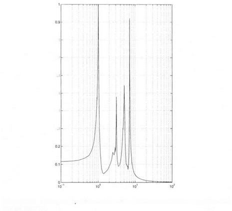
When choosing a sufficiently fine frequency gridding, good results are obtained in many practical examples. A specific problem however arises in the context of flexible systems: indeed, narrow and high peaks may be obtained on the plot of p(M(ju>)) as a function of frequency o> (see Figure 1.17). The use of a frequency gridding is unreliable in such a case: the risk is to miss a peak on the p plot, and to overevaluate the robustness properties of the closed loop (by underevaluating the value of the maximal s. s.v. over the frequency range). In the context of this new and difficult problem, chapter 10 proposes a method for computing a reliable estimate of p{M{ju>)) as a function of u>.

THE SPECIAL CASE OF FLEXIBLE SYSTEMS

0.8


0.7


06


0.5


0.4


03


THE SPECIAL CASE OF FLEXIBLE SYSTEMS

THE SPECIAL CASE OF FLEXIBLE SYSTEMS

THE SPECIAL CASE OF FLEXIBLE SYSTEMS

DIFFICULTIES OF THE ц APPROACH

4.6.1 COMPUTATION OF /x BOUNDS

• Computing the exact value of the s. s.v. is an NP hard problem (Braatz et al., 1994), so that the computational burden of the algorithms, which compute the exact value of /x, is necessarily an exponential function of the size of the problem. It is consequently impossible to compute the exact value of /x for large dimension problems. A usual solution is to compute n upper and lower bounds instead of the exact value. The as­sociated algorithms can be exponential time (like the algorithms which compute the exact value of /x), or more interestingly polynomial time. Even if the gap between the ц bounds can not be guaranteed a priori when using polynomial time algorithms, good results can be obtained in realistic examples: this will be illustrated in the following.

• From a computational point of view, a (skewed) /x upper bound is typically obtained as the solution of a convex or quasi-convex optimiza­tion problem, namely a Linear Matrix Inequality problem (Boyd et al., 1994; Gahinet et al., 1995).

Conversely, methods which compute a /x lower bound are generally heuristic, and the computational burden is required to be low. The most classical solution consists in solving in an heuristic way a non convex optimization problem: a ц lower bound corresponds indeed to a local optimum of this non convex optimization problem, whereas the exact value of /X corresponds to the global optimum of this optimization prob­lem.

The idea is more precisely to obtain the lower bound as the limit of a fixed point iteration Xk+i = f(xk), which is obtained by rewriting the ne­cessary conditions of optimality as f{x) = x (Packard et al., 1988; Young and Doyle, 1990). Note however that the associated power algorithms are not guaranteed to converge, and that the final result depends on the initialization of the fixed point iteration. This will be further detailed in the following. [6]

Д = diag(5ilqi). Remember the unit hypercube D is defined in equa­tion (1.20). An upper bound Д of p{M) gives a sufficient condition of nonsingularity of the matrix I — MA, which is thus guaranteed to be nonsingular for all parametric uncertainties Д inside (1 /JI)D.

Note also that an upper bound Ji of the s. s.v. becomes a lower bound (1/Д) of the m. s.m., so that a lower bound к* of the robustness margin kmax is finally obtained as:

DIFFICULTIES OF THE ц APPROACH

In the context of a robust stability problem in the presence of paramet­ric uncertainties, closed loop stability can thus be guaranteed inside the hypercube kbD in the space of uncertain parameters.

Conversely, a lower bound p of p(M) gives a sufficient condition of singularity of the matrix I – MA, i. e. there exists a real model perturb­ation Д* Є (1 /p)D, with I — MA* singular (in the context of a robust stability problem, Д* is a destabilizing model perturbation).

The usefulness of a p lower bound is twofold. As a first point, p gives a measure of the conservatism of the upper bound p, by examining the tightness of the interval [p, Д] which contains the exact value of p. As a second point, an associated worst-case model perturbation Д * is usually provided with p by the computational algorithm.