More sophisticated methods can be used to move the poles of A + BA*RC through the imaginary axis. In the spirit of (Magni and Doll, 1997), a solution is to introduce an additional model perturbation Ar. The aim is then to find the minimal size model perturbation Дд + Ад, which moves one pole of A + B(A*R -t – Ад)С through the imaginary axis. This problem can be easily recast as a simple Linear Programming problem.
First remember that the model perturbation is diagonal:
Ад = diag(6iIkl, S2lk2i – ■ ■ ,firlkr)
Ад = diag(6lIkl,6*2Ik2,…,6*rIkr) (5.26)
Let A о the closed loop pole, which is the closest to the imaginary axis. Using well-known results on eigenvalues derivatives (Kato, 1980), and assuming that the magnitude of the additional parametric uncertainties Si is sufficiently small, the first order variation of Ao is computed as an affine function of the Sfs:
Г
 *Ao = ^2
1=1
In order to impose that Ao is moved onto the imaginary axis, one imposes 7£e(Ao + <5Ao) = 0. Remember then that the infinity norm of the model perturbation A*r + Ад is to be minimized, so that the problem reduces to the minimization of scalar 7 under the constraints:
 -7 < s* + й <_7, i = l,…,r TZe(Xo + ^2i a(Si) = 0
It may be necessary in practice to modify the above problem, when the eigenvalue Ao is not sufficiently close to the imaginary axis. In this case indeed, the accuracy of the first order development may not be sufficient, to directly move the pole onto the imaginary axis. A solution consists in partitioning the real segment between Ao and the imaginary axis, and to iteratively perform the migration on each sub-segment. At the end of this process, the method of the previous subsection is applied, to ensure an exact pole placement on the imaginary axis.
Remarks:

(/’) In the same way as in (Magni and Doll,
of the model perturbation A*R + Дд could be minimized, instead of the infinity norm. The results are however more conservative than those obtained with the LP method above, since the s. s.v. handles the infinity norm.
(//) It would be possible to impose that the imaginary axis is crossed at a given point juj, in order to compute a lower bound of ^AR(M(juj)) at a given frequency u>. In this case, two equality constraints (7?.e(Ao + £Ao) = 0 and 2m(Ao + <SAo) = u>) instead of a single one (7£e(Ao + £Ao) = 0) are to be considered. Nevertheless, the approach becomes numerically sensitive, since it appears difficult to move the closed loop poles onto
some regions of the imaginary axis (especially at very low and very high frequencies).
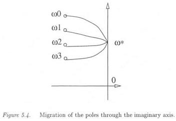
(/77) It is worth emphasizing that the aim is not to compute a lower bound of n at a given frequency, but to detect the peak values on the H plot, in order to directly compute a lower bound of the maximal real s. s.v. over the frequency range. Assume that a ц lower bound was computed for the regularized ц problem at a frequency wo, which is far from the critical frequency ш*. Using especially the LP method above, the imaginary axis can be crossed at a frequency <I>o which is very close to to* (see Figure 5.4). Indeed, the imaginary axis is not constrained to be crossed at a given point jco, and the norm of the model perturbation Дд + Дд is to be minimized. As a consequence, it is generally observed that the imaginary axis is crossed at frequencies which corres
pond to the peak values on the p plot (remember that p is homogeneous to the inverse of the robustness margin, so that the peak values on the p plot correspond to model perturbations which are of minimal size). The method consequently detects the critical frequencies on the p plot: see also chapter 10 (subsection 6.4).
(iv) The following table summarizes the three methods presented above.
|
Table 5.1.
|
Methods for computing a p lower bound.
|
|
Method #
|
Description
|
|
|
1
|
single parameter optimization (a) considering the stability of all poles
|
|
2
|
single parameter optimization (a) considering the stability of one pole
|
|
3
|
Optimization of Д’ using an LP method
|
4. SUMMARY
A great deal of work was devoted to the problem of computing the s. s.v.. Existing computational algorithms can be sorted following various criteria:
■ Nature of the structured model perturbation: two large categories of methods can be considered, corresponding to the special case of a real model perturbation and to the general case of a mixed model perturbation [7].
■ Nature of the result: the algorithm provides the exact value of p, a p lower bound or a p upper bound.
■ Computational requirement: in polynomial time algorithms (resp. exponential time algorithms), the computational amount is a polynomial (resp. exponential) function of the size of the problem. Nevertheless, it must be noted that the computational amount can also largely differ for two methods inside the same category. Remember finally that an algorithm, which computes the exact value of p, is necessarily exponential time, since this problem is NP hard.
|
Table 5.2. Characteristics of the fi computational techniques.
|
Zadeh and Desoer
|
real Ц upper bound
|
exponential time
|
|
Jones
|
real fi upper bound
|
exponential time
|
|
Dailey
|
real /і lower bound
|
exponential time
|
|
a(DMD~l)
|
complex /і upper bound
|
polynomial time
|
|
Fan et al
|
mixed Ц upper bound
|
polynomial time
|
|
Safonov and Lee
|
mixed Ц upper bound
|
polynomial time
|
|
Packard et al
|
complex /і lower bound
|
polynomial time
|
|
Young and Doyle
|
mixed /і lower bound
|
polynomial time
|
|
Magni and Doll
|
mixed /і lower bound
|
polynomial time
|
|
Method of section 3.
|
real p lower bound
|
polynomial time
|
|
As an illustration, the characteristics of the computational methods, which were presented in this chapter, are summarized in the above table. In practice, a trade-off is to be achieved between the accuracy of the result, the computational requirement and the size of the problem. As a simple example, the exact value of jj, can be computed in the case of small size problems, without an excessive amount of computation. However, computing the exact value of /x in the case of medium or large size problems would require an excessive computational amount.
More generally, in the case of small dimension problems, exponential time algorithms can be used. However, it is necessary for large size problems to compute an interval of the s. s.v. j with polynomial-time algorithms. Even if the gap between the ц bounds can not be guaranteed a priori, good results can be nevertheless obtained in realistic examples, as illustrated in chapter 6. Finally, concerning more specifically the computational methods, the following two points are recalled:
■ The mixed fx upper bound by Fan et al is obtained as the solution of a quasi-convex optimization problem, namely an LMI problem.
■ Conversely, the mixed /x lower bound by Young and Doyle is obtained as the solution of a non convex optimization problem: the idea is more precisely to obtain the lower bound as the limit of a fixed point iteration Xk+i = f(xic)- However, the associated power algorithm is not guaranteed to converge, and the final result depends on the initialization of the fixed point iteration. Nevertheless, good results are generally obtained, except in the case of a purely real model perturbation. In this specific context, it is more interesting to use Dailey’s method if the size of the problem is sufficiently small (this method is indeed exponential-time). Otherwise, section 3. proposes a polynomial-time method, which directly computes a lower bound of the maximal s. s.v. over the frequency range.


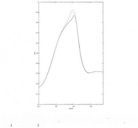 Robust performance is analyzed in the frequency domain, using the sensitivity function S (see section 2. of chapter 2 for the definition of S). A fictitious performance block is added to the model perturbation, which now contains 4 non repeated real scalars and a full complex block.
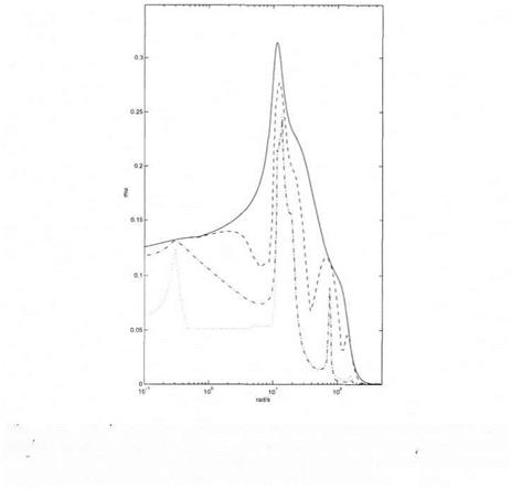 Missile autopilot – robust stability inside a truncated sector (P2) – the
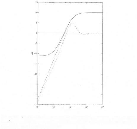 the presence of uncertainties in the aerodynamic model.
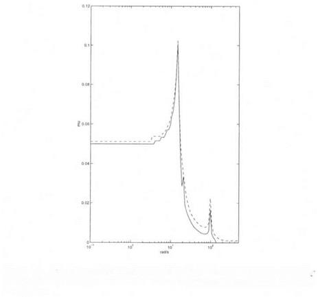 Figure 6.1. Missile autopilot – robust stability (PI) – the real p upper bound b
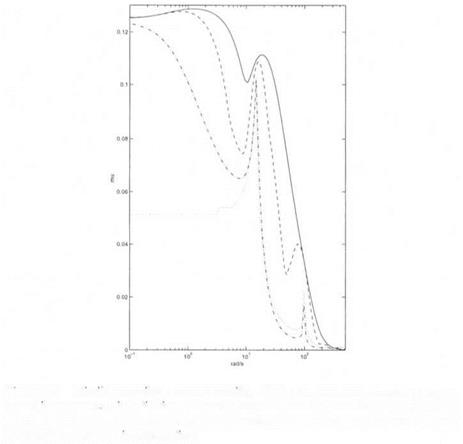 Missile autopilot – robust stability (PI) – the classical complex /і upper
 p(M) = гам pr(AM)
 ц{М) = шxpR(QM)