Category BASIC AERODYNAMICS

In the previous sections, introductions to the problem of modeling fluid flows in aero­dynamics and some calculations for aerodynamic forces are presented. At several points, information about properties of the atmosphere are required in completing the calculations. For example, it is frequently the case that we need to know the value of the atmospheric temperature, density, or pressure when estimating the magnitude of aerodynamic forces or evaluating propulsion-system performance. This need pro­vides the opportunity to gain further practice in handling fluid-mechanics modeling
and, in the process, to review methods for representing atmospheric effects. Because only the simplest type of physical relationship is involved, we can accomplish this now without using the more sophisticated modeling needed in subsequent problems. Only the ideas of statics and the ideal gas equation are required.

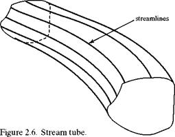
In addition to visualization, there are other useful applications of streamlines. Con­sider, for instance, a bundle of streamlines that pass through a reference volume of arbitrary shape and size. The outermost set of streamlines form the walls of a stream tube and define the surface. Figure 2.6 shows a length of a typical stream tube. If the cross-sectional area of a stream tube is small, it is often referred to as a stream filament. The “streamlines” in an experiment using smoke for flow visualiza­tion in reality are stream filaments because the smoke must be injected from orifices of small but finite size. Obviously, all the streamlines passing through neighboring points must be nearly parallel, although they may diverge or become even more closely packed farther downstream.

Because there is no flow across any streamline, a stream filament behaves as a miniature pipe. We show in the next chapter that the average velocity at any point along a stream tube or stream filament is related to its cross-sectional area. It is almost obvious that if the flow is incompressible, the speed must increase when the area decreases and vice versa.

Of the visualization lines described previously, the streamlines have the most value as a flow-visualization device throughout this book. This is because for the most part, we concentrate on steady-flow applications. Because streamlines are such a useful tool, we now must learn how to describe them mathematically.

Suppose that we have carried out an analysis for a flow problem that results in a solution for the velocity vector as a function of position in an appropriate coordi­nate system. That is, we found the velocity vector throughout the domain in Eulerian form:

V = V(r, t),

where r is the position vector for any point in the domain. This might be a compli­cated algebraic function that is difficult to interpret physically. Mathematical flow visualization is necessary to bring out the details. To illustrate the method, consider a case in which V is described in terms of a Cartesian coordinate system in which a point in the flow is identified by its position vector, r = xi + yj + zk, where i, j, and k are the unit vectors along the three coordinate axes. Then, in component form,

V = u(x, y,z, t)i + v(x, y,z, t)j + w(x, y,z, t)k,

where u, v, and w are the velocity components as a function of position in the field. How can we find the streamline for this velocity vector that passes through a given point? By definition, the streamline must be parallel to the velocity vector. There­fore, the slope of the streamline projected on each of the three planes normal to the coordinate directions must be equal to the slope of the projection of the velocity vector. Thus, we must have:

dy = v dz = w dz = w dx u dx u ’ dy v

as the condition of tangency at any given time. Because these can be written in the form:

dy = dx dz = dx dz = dy v u ’ w u ’ w v

it is clear that this information can be conveyed best in the simpler form:

dx = dy = dz u v w ‘

To find the equation of the streamline at an instant of time, it is necessary to inte­grate these equations to define, for example, z = z(x, y), which is an equation for any streamline. To find a particular streamline, which can be plotted for flow visualiza­tion, we simply evaluate the constants of integration by inserting values of x, y, and z corresponding to a point through which that streamline passes.

This is a simple process for two-dimensional problems because we then must integrate only the simple equation:

dy = v dx u

to find y = y(x), which describes the required streamline.

The following example illustrates the technique used in finding a mathematical description of streamlines in a given flow. Notice that the presence of a function of time is of no concern because only the instantaneous streamline is meaningful.

EXAMPLE 2.5 Required: Find the equation for streamlines in a flow field described by the unsteady velocity vector:

V = x(1 + at2)i + yebtj.

Find the specific streamline passing through the point (3, -2) at time t = 0. Approach: Integrate Eq. 2.26.

Solution: Substituting the velocity components into Eq. 2.26 yields:

dy = v = ye

dx u x(l + at2)’

The equation is separable so, for a given time, we can write:

which immediately can be integrated to give:

where C is the constant of integration. Notice that the streamline is time – dependent. Because we want the streamline passing through point (3, -2) at time t = 0, C is readily found to be C = -2/3, and the required streamline equation is:

which is obviously a straight line at t = 0. The shape of the streamline changes as time progresses unless constants a and b are both zero.

One characteristic of fluid flow that makes it challenging to study is that in most cases, unlike solid mechanics, the medium is invisible. Experimental fluid mechanics makes use of smoke or dye to obtain visual insight into the physics of a flow. Like­wise, it is helpful in analysis to obtain an analogous mathematical “visual” represen­tation of a flow field whenever possible. The following three types of flow lines are of great value in flow visualization:

1. Streamlines. These lines are everywhere tangent to the velocity vector. They are most useful in describing a steady flow because in that case, each stream­line is the path that a fluid particle traces as it traverses the flow field. In an unsteady flow, the velocity vector changes in both direction and magnitude with time at any given point; therefore, only instantaneous streamlines are useful in visual interpretation of the field. That is, they describe how fast and in what direction the fluid particles are moving at a given instant. Because streamlines are always parallel to the velocity vector, flow cannot pass across a streamline.

2. Streaklines. These lines would be traced out by a marker fluid that is con – tinuosly injected into the flow stream at a given point. This is a commonly used experimental flow-visualization technique. For example, smoke often is injected into a flow to make the details visible. If the flow is steady, the fil­aments of smoke particles trace out the streamlines that pass through the injection points.

3. Pathlines. These are lines traced out in time by a given particle as its motion would be explained in a Lagrangian mathematical description.

The physical laws evoked in derivation of the defining equations all apply to a system (e. g., recall that the First Law of Thermodynamics refers to a system). A system is

Figure 2.5. Fixed finite control volume.

a collection of fluid particles of fixed identity. Visualize a sealed plastic bag filled with liquid or gas that is proceeding downstream in a flow. The contents of the bag constitute a system. Note that if the flow is compressible, the density of the material inside the sealed bag may change. That is, the volume enclosed by the plastic bag may change but the mass of material contained within the bag must remain constant. A system may be finite in size or infinitesimal. An infinitesimal mass of fluid of fixed identity is termed a fluid particle.

Control Volume

The fundamental physical laws or principles expressing conservation of mass, momentum, and energy are expressed with respect to a system, as previously men­tioned. For example, the First Law of Thermodynamics states that the heat added to a system minus the work done by the system equals the change in internal energy of that system. In aerodynamics, however, it is more convenient to derive these conser­vation equations by applying the physical laws to a control volume rather than to a system.

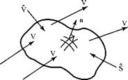
A control volume is a volume fixed in space. Flow may pass into or out of the control volume through the control surface that surrounds the control volume. Con­sider a surface that encloses a volume of arbitrary shape. Imagine that this surface is made of wire screen and that it is fixed in space in a flowing medium. Fluid may pass in or out through the porous screen, as illustrated in Fig. 2.5. The wire screen constitutes a control surface enclosing a control volume. This control volume may be finite or infinitesimal in size.

Review the definition of a system; it is different than a control volume, and the two concepts must be clearly understood. Both have important applications because the mathematical tools needed for describing a flowing medium are derived in sub­sequent chapters.

Several concepts of great value in later derivations of the defining equations are reviewed in this section. It is important that students are familiar with these ideas, especially the mental images that they require. Students probably are already fami­liar with some or all of these ideas from their fundamental courses in mechanics or thermodynamics.

Lagrangian versus Eulerian Mathematical Description

In studying the motion of particles and rigid bodies in mechanics courses, students learned the Lagrangian approach in which each element of the system is represented by a detailed model of its absolute motion and its motion relative to other parts of the system. In aerodynamics (or fluid mechanics), two different mathematical viewpoints may be adopted. Following the Lagrangian methods used in mechanics, physical laws are applied to individual particles in a flow. Equations then are derived that pre­dict the location and status of individual fluid particles as a function of time as they move through space. The equations of dynamics typically use the Lagrangian view­point, time being the only independent variable. In these situations, it is necessary to keep track of the positions and velocities of all elements that comprise the system. However, for fluid-flow problems, so many particles are involved (virtually, an infinite number) in the field that this modeling stratagem usually is not practical.

Aerodynamics is concerned with a continually streaming fluid and the task is to determine distributions of flow velocities and fluid properties within a flow-field region rather than tracking the motion of specific particles passing through the region. For example, pressures at the surface of an airfoil or at points of interest in the flow are the main concern, not the behavior of the individual particles that exert these pressures. For this reason, a field, or Eulerian, representation is preferred in most aerodynamics problems and this viewpoint is taken herein. In this rep­resentation, the fluid properties and velocities throughout the flow are expressed in terms of position and time. Thus, flow variables such as pressure and velocity are described in terms of the flow-field coordinates and time, so that for an unsteady flow in 3-dimensional Cartesian coordinates (x, y,z), the pressure p = p (x, y,z, t) and the velocity vector V = V(x, y,z, t).

We already discussed geometrical similarity. In conducting experiments using scale models to determine force coefficients, it is clear that both the shape and orientation relative to airflow are important. However, suppose that we accurately measure the lift coefficient under conditions of geometric similarity on a model, for example, one-tenth the size of the actual vehicle. Is this enough? Can we now use this lift
coefficient to estimate the lift on the prototype? The results of Eq. 2.22 show that this might not work. We must conduct the test so that the Reynolds and the Mach numbers on the model match those on the prototype. If this is done, we will achieve dynamic similarity and the predictions most likely will work if we correctly identi­fied all of the key variables.

This is a concept of enormous value in the planning of experiments. Notice that even a complete theory or a complete numerical study often must be verified by experiments. It is therefore crucial to do this in a cost-effective and efficient manner. The principle of dynamic similarity is the key. In the wing-design example in the previous subsection, it is clear that if we had known the flight Reynolds and Mach numbers for the prototype, we would be able to design a test matrix that held these quantities fixed; the number of required test conditions could be reduced drastically.

It may not always be easy to match both the test Reynolds and Mach numbers to the prototype values. For instance, in testing a model of a hypersonic airplane, to fly at a Mach number of, for example, M = 11, configuring the test apparatus using a small model (no large wind tunnels can operate continuously in this Mach-number range) probably would lead to a Re that is too small to match that experienced on the full-sized prototype. However, it often may be the case that one or more of the similarity parameters is of lesser importance. In the hypersonic airplane example, it may be that dependence on viscous effects is secondary to compressibility effects, which are important in high Mach-number flight. Then, useful data still can be obtained without a matching Re. What is required here is an intimate knowledge of the sensitivity of the results to the parameters involved. This knowledge comes with experience. We attempt throughout this book to aid the student in acquiring at least some of the needed experience.

EXAMPLE 2.4 Situation: A 1:10 scale model sailplane wing is tested in a wind tunnel to determine the aerodynamic characteristics. The span of the prototype is 15 m and the average chord (width) of the wing is 0.8 m. Sea-level air is the working fluid for both the model and full-sized wings.

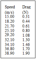
Data from the test are shown in the table.

Required: (1) Sensitivity of the drag coefficient to the Re based on the average chord length; and (2) drag estimate for the prototype at a speed of 135 km/hr.

Approach: Use the dynamic similarity principle. If the drag coefficient can be shown to be insensitive to the Re, then the model data can be applied directly in estimating the drag.

Solution: The drag coefficient can be found from:

D

m

2P [6]mSm

where the subscript, m, refers to the model. Standard sea-level air has a density

0 8 15

of 1.23 kg/m3, and the area of the model wing is S = — x — = 0.120 m2.

m 10 10

which is dimensionally correct if the drag measurements are inserted in newtons (N) and the velocity is measured in m/s.

Because the kinematic viscosity for sea-level air is:

2

M. . _ . n-5 m v = — = 1.45 x 10 5 —,

P ^

the Re for the model based on the average chord is found from:

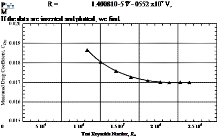
This shows that above a Re of about 1.5 x 105, the drag coefficient is insensi­tive to the Re (this may break down at yet higher speeds). This corresponds to a speed of about 27 m/s. Therefore, above this value, the drag coefficient has a nearly constant value of about CD = 0.017. If the prototype speed is: V

Appraisal: This example illustrates several useful features of the dynamic – similarity approach. It often happens that the aerodynamic force is insensitive to one or more of the similarity parameters. In this case, the Reynolds-number dependence was weak in the speed range of interest. Therefore, the drag coefficient measured in the wind tunnel could be used directly. Notice that there was no men­tion of possible Mach-number dependency; this is because the speed range is so low compared to the speed of sound that compressiblity effects are unimportant.

Using these ideas, a helpful way to write the expression for the aerodynamic force is:

F = C(M, Re)pV2d2, (2.21)

where the effects of the dimensionless groups now have been incorporated into a coefficient of proportionality, C. For example, what is usually written in aero­dynamics problems involving, for example, the lift and drag on an airplane wing is:

where the coefficients CL(M, Re) and CD(M, Re) are functions of the appropriate similarity parameters. These are the well-known lift and drag coefficients, respec­tively. The factor of 1/2 is introduced here to take advantage of the fact that the combination

dynamic pressure = q =[3] pV[4] [5],

which has the dimensions of pressure, appears throughout the book as an important aerodynamic parameter. The area, S, is introduced as a convenient substitute for the squared characteristic length, d, which clearly has units of area. Any convenient reference area can be used.

In the study of lift on three-dimensional wings, the reference area, S, usually is chosen as the projected area of the wing surface. Other choices can be made. For instance, in describing the drag of bodies of revolution, we often use the projected frontal area of the body as the reference area, S.

Notice that, by using a combination of physical and dimensional reasoning, we now have reduced the aerodynamic-force problem to a convenient and practical form, which can be applied readily in airplane design, for instance.

Consider the application of Eq. 2.22 for determining, for example, the lift on an airplane wing. Three main elements are involved. One factor, the dynamic pressure, describes the environment—that is, the flight speed and altitude as represented by air density (which, as we shall see, is strongly dependent on altitude). An important geo­metrical dependence is seen in the reference area, S. Finally, a coefficient, CL, implies a dependence on compressibility and viscous effects because, as demonstrated, its value is a function of the Mach and Reynolds numbers characterizing the flow field. It must be understood that aerodynamic coefficients also are dependent on geometry.

The situation would be simplified if the coefficients were thought of as constants. Then, it would be necessary to compute or measure them only once for a given shape to provide design information for using that shape in a practical application. How­ever, our analysis shows that they vary with special parameters—in this case, the Reynolds and the Mach numbers.

To use Eqs. 2.22-2.23, for example, in a wing-design problem, we must have values for all three factors. The first two are known from the design operating con­ditions and the geometry. However, how can we determine the lift coefficient? Sev­eral approaches naturally come to mind:

Why are there different approaches and how do we determine which is the cor­rect one to use in a given situation? These are important practical questions, and we endeavor to provide the answers in the following discussion. A major objective of this book is to introduce methods for accomplishing Method 1. An introduc­tion to Method 2 also is discussed in considerable detail at approprate points. The numerical approach is rapidly gaining in popularity as large-scale computing costs drop and workstation and desktop computer capabilities improve. Method 3, experi­mentation, is the traditional approach and still is used extensively for reasons that will become clear. It is also important to observe the relationship between Methods 2 and 3. In many ways, Method 2 is another method of experimentally determining the required information. It represents “virtual” experimentation, which can take the place of a usually more costly physical experiment.

It is of the greatest importance that the student realizes that experimentation, either numerical or physical, cannot be used as a substitute for a thorough theor­etical understanding of the problem to be solved. The flow-similarity ideas discussed in this chapter show how important this physical understanding can be. Even lacking an in-depth theory of gas flow over a body, using simple dimensional reasoning, we have identified the correct relationship between the key variables in Eqs. 2.22 and 2.23 for determining aerodynamic forces. Basically, it reduces the problem to one of finding coefficients such as CL and CD.

To illustrate how important such theoretical results can be, consider the following example: Suppose it is your job to design the wing of a new airplane. You consider yourself an experimentalist and do not have much use for theoreticians and their incessant equations. However, you fully understand the thinking that led to Eq. 2.10. You know that there are five key variables. You also understand geometrical simi­larity, so you proceed to build a scale model of the airplane to be tested in the wind tunnel. Now, if you are not armed with the right theoretical understanding, you prob­ably will think that it is necessary to vary all five of the variables to obtain a full set of data describing how the forces on the wing vary with speed, density, viscosity, size, and so on. If it takes a minimum of five values of each variable over their expected range to determine how they affect the aerodynamic forces, then it is easy to see that it will require 55 = 3,125 separate test runs to acquire the needed information. Keeping in mind the high cost of laboratory space, instrumentation, and technicians, this would turn out to be an expensive and time-consuming exercise; you would most probably lose your job.

Conversely, if you base your experiments on your understanding of the theory, you will see that there are only two parameters to keep track of on a model shaped and oriented like the real prototype: the Reynolds number and the Mach number. The number of experiments needed can be reduced drastically.

Any physical problem can be analyzed in the manner just illustrated. It always hap­pens that dimensional reasoning alone cannot show in detail how each parameter (e. g., the viscosity or speed of sound) enters the mathematical expression governing the problem. However, the dimensionless groupings that appear have enormous sig­nificance. Hundreds of these groups have been identified as important in engineering applications; they usually are assigned the name of the individual who first recog­nized its importance. For example, in the aerodynamic force expression derived in Eq. 2.14, the two groups that appear are as follows:

The first group was identified as a key parameter in describing the effects of compressibility in aerodynamic flows. It was introduced by the Austrian physi­cist Ernst Mach in the 1870s. The second is named for Osborne Reynolds, who showed in the 1880s that this group governs the role of viscous forces in the flow of liquids or gases. In particular, it controls the transition between laminar and turbulent flow.

Each dimensionless group can be identified as the ratio of sets of forces gov­erning the fluid flow. Clearly, the ratio of any two such forces is a dimensionless number like those we found. Some key forces are:

where the dimensional form is expressed by means of the notation introduced in Table 2.2. Thus, the ratio:

inertia force = [pV2!*2] viscous force " WL]

is the Reynolds number. All dimensionless groups can be expressed similarly as ratios of the forces governing the fluid motion. Table 2.3 lists a set of forces and their dimensions that may occur in fluid-dynamics problems. Of these, only the viscous force, pressure force, and force related to compressibility are likely to be encoun­tered in aerodynamics problems.

It is important to demonstrate the power of the concept of similarity param­eters. Using the Reynolds number to illustrate, consider what the difference would be in a flow with a high Re compared to one with a low Re value. For example, the flow over an airplane wing in low-speed flight typically has a Re number (based on the flight speed and average width of the wing) of two million or three million. From Eq. 2.20, it is clear that this means that the inertia forces—those due to acceleration or deceleration of gas particles moving over the wing—are enormous compared to the viscous forces due to the shearing stresses along the surface. For a second example, consider the flow of ketchup from an upturned bottle. Here, the Re is small, indicating the overwhelming importance of the viscous forces in controlling the flow.

With the simple tools now at our disposal, we can gain considerable insight into the nature of aerodynamic forces and related flow-field effects. A powerful tool is the requirement for dimensional homogeneity. This makes it possible to uncover relation­ships between parameters without complete information about the actual physics of any underlying phenomena, which may not be known at the outset. The method we now construct has many applications, not the least important of which is the planning and implementation of experimental studies of complex aerodynamic phenomena.

We return now to the ideas expressed in Eq. 2.8. We expect that on the basis of our observations, the drag force is a function of several flow parameters and on the geometrical configuration of the object immersed in the gas flow. This is true for any aerodynamic force component, F, so let us generalize by writing:

F = F(V, p, p, a, d), (2.10)

where we now have chosen a set of parameters that reflect our expectations that speed, V; gas density, p; and size may affect the force. We also include the speed of sound, a, and the coefficient of viscosity to account for possible compressibility and shear-force effects. The pressure is excluded because the force is clearly the result of pressure distribution over the body; to include it simply would double the depen­dence on the same quantity. The influence of the size of the object is reflected by inclusion of a length d, which could be any one of the dimensions of the object (e. g., length or width). A parameter describing the shape is not incorporated because it is not possible to represent this by a mathematical parameter. Instead, we employ the concept of geometric similarity. The relationship to be constructed holds for any family of objects, possibly of different sizes but with the same shape (as illustrated in Fig. 2.4)—that is, a family of similar shapes.

We now examine Eq. 2.10 from the standpoint of dimensional reasoning. The method to be used often is generalized in an elegant form known as the Buckingham Pi Theorem. The full machinery is not needed at this point in the discussion; a sim­pler intuitive approach is more instructive as an introduction.

The first step is to choose an appropriate mathematical form for the relation­ship implied in Eq. 2.10. To accomplish this, we simply note that in the majority of such situations, physical relationships involving several variables are in the form of products of powers of the several variables. There is no guarantee that this will work here; however, subject to subsequent careful analysis, we ask what such a relation­ship would yield in the current problem.

With this in mind, assume that the aerodynamic force F is a function of products of the several variables to unknown powers. This choice is based on the observation that mathematical descriptions of natural phenomena often take this form. Write:

F = CVc p°2 pc3 a°4 d°s,

Figure 2.4. Geometric similarity. All shapes shown are identical, although sizes are different. Because

(b)

(a)-(c) also are oriented at the same angle to the reference line, they are geometrically similar.

(c) Shape (d) is identical to (a), but it is oriented differently with respect to the reference line. Therefore, shape (d) is not geometrically similar to the other shapes.

(d)

where C is an arbitrary (i. e., dimensionless) constant and cn (n = 1 to 5) is a set of initially undetermined exponents. Thus, in terms of the dimensions of each of the six factors, it is necessary for dimensional homogeneity that:

where the mass-based set defined in Table 2.2 is used. The same results would be forthcoming if the force-based dimensions were used instead. Now, for Eq. 2.11 to be dimensionally correct, it is necessary that each of the three basic units enters the problem with the same exponent on each side of the equation. Therefore, for dimen­sional homogeneity, it is necessary that 1

Therefore, the aerodynamic force can be written as:

F = СУ(2_Сз-С4)р(1-Сз)цСз a4 d(2-°3).

Collecting the terms with the same unknown exponent, we find:

(2-14)

It is not possible to determine the exponents c3 and c4 using dimensional homogeneity alone. However, the expression we found contains vital information regarding the dependence of the aerodynamic forces on the parameters that we identified as those most likely to matter. Notice that the expressions raised to the powers c3 and c4 are dimensionless groups of the variables. Because the exponents are unknown, it would be correct to rewrite Eq. 2.14 as:

where two new exponents (d3 and d4, which are obviously the negative values of the original two) are used. The two dimensionless groups clearly have physical significance in the system behavior. They are called similarity parameters and are the focus of considerable attention throughout this book. One of the param­eters, arising in a natural way in this simple analysis, is the Mach number V/a that was encountered in the introduction to compressibility effects previously in this chapter. The second, called the Reynolds number, clearly is related to effects of viscosity.