Category COMPUTATIONAL AEROACOUSTICS

If the fourth-order approximation of Eq. (1.23) is used instead of Eq. (1.22), it is easy to show that the governing finite difference equation for йе is

The two physical boundary conditions of Eq. (1.15) are

й0 = 0, йм = 0. (1.35)

Now, Eq. (1.34) is a fourth-order finite difference equation. There are four linearly independent solutions. In order to have a unique solution, four boundary conditions are necessary. However, only two physical boundary conditions are available. To ensure a unique solution of the fourth-order finite difference equation, two extra (nonphysical) boundary conditions need to be created. Also, two of the four solutions of Eq. (1.34) are spurious solutions unrelated to the physical problem. Therefore, the use of high-order approximation will result in

(A) Possible generation of spurious numerical solutions.

(B) A need for extra boundary conditions or special boundary treatment.

These are definite disadvantages in the use of a high-order scheme to approximate partial differential equations. Are there any advantages? To show that there could be an advantage, note that the eigenfunction of the finite difference equation (1.33) is identical to the exact eigenfunction (1.21). As it turns out, the eigenfunction (1.33)

Figure 1.3. Comparison of normal mode

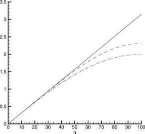frequencies. _________ , exact, Eq.

(1.20);————– , fourth-order, Eq.

(1.37);…… , second-order, Eq. (1.32).

of the second-order approximation is also the eigenfunction of the fourth-order approximation, namely, the solution of Eqs. (1.34) and (1.35) is

Щ = sin( , n = 1 2, 3,…. (1.36)

These eigenfunctions satisfy boundary conditions (1.35). On the substitution of solu­tion (1.36) into Eq. (1.34), it is easy to find that the corresponding eigenfrequency is given by

It is straightforward to find that frequency formula (1.37) is a much improved approximation to the exact eigenfrequency of formula (1.20) than formula (1.32) of the second-order method. Figure 1.3 shows a comparison for the case M = 100. This result illustrates the fact that, when the problems of spurious waves and extra boundary conditions are adequately taken care of, a high-order method does give more accurate numerical results.

On replacing the spatial derivative of Eq. (1.15) by Eq. (1.22), the finite difference equation to be solved is

Eq. (1.24) is a second-order finite difference equation, the same order as the original partial differential equation. For a unique solution, two boundary conditions are required. This is given by the boundary conditions of the physical problem, Eq. (1.14); i. e.,

u0 = 0, uM = 0. (1.25)

On following Eq. (1.16), a separable solution of a similar form is sought,

U (t) = Re [Uee-lmt]. (1.26)

Substitution of Eq. (1.26) into Eqs. (1.24) and (1.25) leads to the following eigenvalue problem:

U0 = 0, UM = 0.

Two linearly independent solutions of finite difference equation (1.27) in the form of Eq. (1.4) can easily be found. The characteristic equation is

The two roots of Eq. (1.29) are complex conjugates of each other. The absolute value is equal to unity. Thus, the general solution of Eq. (1.27) may be written in the following form:

Ue = A sin (©l) + B cos (©l).

where

Upon imposition of boundary conditions (1.28), it is easy to find

B = 0, A sin (©M) = 0.

For a nontrivial solution, it is required that sin(0M) = 0. Hence,

&M = nn, n = 1, 2, 3,…

or

This yields

Now, it is instructive to compare finite difference solutions (1.32) and (1.33) with the exact solution of the original partial differential equations (1.20) and (1.21). One obvious difference is that the exact solution has infinitely many eigenfrequencies and eigenfunctions, whereas the finite difference solution supports only a finite number (2M) of such modes. Furthermore, mn of Eq. (1.32) is a good approximation of the exact solution only for nn/M < 1. In other words, a second-order finite difference approximation provides good results only for the low-order long-wave modes. The error increases quickly as n increases.

Now consider solving the normal mode problem by finite difference approximation. For this purpose, the tube is divided into M equal intervals with a spacing of Ax = L/M as shown in Figure 1.2. l is the spatial index (l = 0 to M). Both second – and fourth-order standard central difference approximation will be used.

To find the normal acoustic modes of the tube, consideration will be given to solutions of the form:

и (x, t) = Re[U(x)e ш],

where Re[] is the real part of [ ]. Substitution of Eq. (1.16) into Eqs. (1.15) and (1.14) yields the following eigenvalue problem:

The two linearly independent solutions of Eq. (1.17) are

U (x) = A sin —J + B cos —J. On imposing boundary conditions (1.18), it is found that

B = 0, and A sin ^-“j = 0- For a nontrivial solution A cannot be zero, this leads to,

Therefore, (1.20)

is the eigenvalue or eigenfrequency. The eigenfunction or mode shape is obtained from Eq. (1.19); i. e.,

. /nnx „ „ „

un (x) = sin ^~l) , n = 1, 2, 3, -.

A concrete example will now illustrate the inherent difficulties of using the finite dif­ference solution to approximate the solution of a boundary value problem governed by partial differential equations.

Suppose the frequencies of the normal acoustic wave modes of a one­dimensional tube of length L as shown in Figure 1.1 is to be determined. The tube has two closed ends and is filled with air. The governing equations of motion of the air in the tube are the linearized momentum and energy equations, as follows:

d u d p

P0 — + — = 0

0 dt dx

d p d U

It + Y P0 dx = °’

where p0, p0, and y are, respectively, the static density, the pressure, and the ratio of specific heats of the air inside the tube; and u is the velocity. The boundary conditions are

At x = 0, L; u = 0.

Upon eliminatingp from (1.12) and (1.13), the equation for u is

d2u 2 d2u

9U – a dX2 = 0’

where a = (yp0/p0)1/2 is the speed of sound.

Since the coefficients of the characteristic polynomial are real, complex roots must appear as complex conjugate pairs. Suppose r and r* (* = complex conjugate) are roots of the characteristic equation; then, corresponding to these roots the solutions may be written as

y^^, У2}=(г* )к.

If a real solution is desired, these solutions can be recasted into a real form. Let r = Rei0, then an alternative set of fundamental solutions is

у{1 = R cos (кв), у(к> = Як sin (кв).

If r and r* are repeated roots of multiplicity m, then the set of fundamental solutions corresponding to these roots is

ук) = Як cos (кв) yf+У = R sin (кв)

yk) = кЯк cos (кв) у{к"+2) = кЯк sin (кв)

к . к. (1.11)

у(т) = кт-1^ cos (кв ) ykm) = к“-1^к sin (кв ) .

example. Find the general solution of

yk+2 – 4yk+1 + 8yk = 0

The characteristic equation is

r2 – 4r + 8 = 0.

The roots are r = 2 ± 2i = 2V2 e±l(n /4). Therefore, the general solution (can be verified by direct substitution) is

yk = A(2V2)k cos kj + B(2V2)k srn(|kj,

where A and B are arbitrary constants.

Now consider the case where one or more of the roots of the characteristic equation are repeated. Suppose the root r1 has multiplicity m1s the root r2 has multiplicity m2, and the root rt has multiplicity mt such that

m1 + m2 +——- -me = n. (1.8)

The characteristic equation can be written as

(r – r1 )m1 (r – r2 )m2… (r – rl )mi = 0. (1.9)

Corresponding to a repeated root of the characteristic polynomial (1.9) of multiplic­ity m, the solution is

ук = (A1 + A2k + A3k ————— Amk>n ^ r, (1.10)

where A1, A2,…, Am are arbitrary constants.

example. Consider the general solution of the equation

Ук+2 – 6Ук+1 + 9Ук = 0.

The characteristic equation is

r2 – 6r + 9 = 0 or (r – 3)2 = 0.

Thus, there is a repeated root r = 3, 3. The general solution is

Ук = (A + Bk) 3к.

If the characteristic roots of Eq. (1.5) are distinct, then a fundamental set of solutions is

yk = k i = 1, 2,…, n

and the general solution of the homogeneous equation is

yk = c1rk + c2rk + ••• + cnrt (1.7)

where cx, c2,…, cn are n arbitrary constants. example. Find the general solution of

yk+3 – 7yk+2 + 14yk+1 – 8yk = °-

Let yk = crk. Substitution into the difference equation yields the characteristic equation

r3 – 7r2 + 14r – 8 = 0

or

(r – 1) (r – 2) (r – 4) = 0.

The characteristic roots are r = 1, 2, and 4. Therefore, the general solution is

yk = A + B2k + C4k,

where A, B, and C are arbitrary constants.

Linear difference equations with constant coefficients can be solved in much the same way as linear differential equations with constant coefficients. The characteristics of the two types of solutions are similar but not identical.

Consider the nth-order homogeneous finite difference equation with constant coefficients:

yk+n + a1yk+n-1 + a2yk+n-2 + + anyk = 0, (1.3)

where ax, a2,…, an are constants. The general solution of such an equation has the form:

Ук = crk, (1.4)

where c and r are constants. Substitution of Eq. (1.4) into Eq. (1.3) yields, after factoring out the common factor crk,

f (r) = rn + a1rn-1 + a2rn-2 +—————– + an-1r + an = 0. (1.5)

Here, f(r) is an nth-order polynomial and thus has n roots ri, i = 1,2,…, n. For each ri we have a solution:

yk = cirk> (1.6)

where ci is an arbitrary constant. The most general solution may be found by super­position.

In this chapter, the exact analytical solution of linear finite difference equations is discussed. The main purpose is to identify the similarities and differences between solutions of differential equations and finite difference equations. Attention is drawn to the intrinsic problems of using a high-order finite difference equation to approx­imate a partial differential equation. Since exact analytical solutions are used, the conclusions of this chapter are not subjected to numerical errors.

1.1. Order of Finite Difference Equations: Concept of Solution

Domain: In this chapter the domain considered consists of the set of integers k = 0,

±1, ±2, ±3,____ The general member of the sequence…, y-2, y_1, y0, y1, y2,… will

be denoted by yk.

An ordinary difference equation is an algorithm relating the values of different members of the sequence yk. In general, a finite difference equation can be written in the form

yk+n = F^k+n-V yk+n-2’ •••> yк k)> (L1)

where F is a general function.

The order of a difference equation is the difference between the highest and lowest indices appearing in the equation. For linear difference equations, the number of linearly independent solutions is equal to the order of the equation.

A difference equation is linear if it can be put in the following form:

yk+n + a1 (k) yk+n-1 + a2 (k) yk+n-2 + •••+ an-1 (k) yk+1 + an (k) yk = Rk> (1.2)

where a(k), i = 1, 2, 3,…, n and Rk are given functions of k.

EXAMPLES

(a) yk+1 – 3yk + yk-1 = 6e-k (second-order, linear)

(b) yk+1 = y2k (first-order, nonlinear)

(c) yk+2 = sin(yk) (second-order, nonlinear)

The solution of a difference equation is a function yk = ф(^ that reduces the equation to an identity.

1