Category COMPUTATIONAL AEROACOUSTICS

The analysis of the previous sections is primary for one-dimensional waves. However, it can easily be generalized to waves in two or three dimensions.

Suppose the multidimensional dispersion relation of a wave system is

Again, assuming there is a simple pole on the real «-axis given by«(ai), it is straight­forward to obtain by the Residue Theorem that the contribution of this pole to the solution is

The triple integral may be evaluated asymptotically for large t by the method of stationary phase in multidimensions. Thus,

where

In Eq. (4.38), det is the determinant of and g depends on the number of factors of n/4 arising from path rotation. Now Eq. (4.39) gives the group velocity, Vi, in three dimensions as follows:

It is easy to see, for a multidimensional finite difference system, that the same analysis applies. Therefore, the conclusions concerning numerical dispersion and dissipation
obtained for a one-dimensional system are also true for multidimensional finite difference approximations.

EXERCISES 4.1. Suppose the initial value problem,

^ + c^r = 0, u(x, 0) = f (x),

dt dx

is computed by approximating the du/dx term by a finite difference quotient, show

(i) If the standard sixth-order central difference approximation is used, the numerical solution can only have trailing waves.

(ii) If the 7-point stencil DRP scheme is used, the numerical solution may have both leading and trailing waves. Estimate the wavelength of the leading waves.

4.2. In solving the convective wave equation,

d U d U

—– + C = 0,

d t dx

by approximating the spatial derivative by finite difference quotient and marching the solution in time by the fourth-order RK scheme, it has been shown that the solution, in wave number space, is governed by the equation

4

1 + ^2 Cj (-icaAt)), j=1

where a(a) is the wave number of the finite difference scheme and n is the time level. One may consider this as a first-order finite difference equation in n (see Chap­ter 1). Find the exact solution of this finite difference equation. To avoid numerical instability, the absolute value of the characteristic root must be smaller than 1.0. Suppose a is the wave number of the standard sixth-order central difference scheme and Cj’s are the coefficients of the standard fourth-order RK scheme. Determine the largest time step At that may be used without encountering numerical instability.

Discretization of a partial differential equation into a finite difference equation, in general, leads to numerical dissipation in addition to numerical dispersion. To illustrate this, again consider solving the convective wave equation (4.11) using a large-stencil finite difference scheme. Suppose the spatial derivative is approximated by a finite difference quotient and solve time exactly. The exact solution of the semidiscretized problem is given by Eq. (4.21) and, upon evaluating the m-integral, the solution is given by Eq. (4.23).

TO

u(x, t) = J Ф(a)ei(ax-ca(a)t]da. (4.33)

— TO

Now, whether the numerical solution is damped or not depends critically on whether a central difference stencil or an unsymmetric difference stencil is used. If a central difference stencil is used, then a(a) is a real function for real a. In this case, Eq. (4.33) represents a dispersive wave packet without being damped in time. If an unsymmetric stencil is used, then a(a) is complex for real a. In this case, the solution is damped in
time provided that Im(ca) is negative for all a. The time rate of damping for the wave component with wave number a is given by c Im[a(a)]. For many popular numerical schemes c Im(a) is negative. Such schemes have built-in numerical damping. The damping rate can be calculated precisely once the stencil size and stencil coefficients are known.

It is worthwhile to point out that it is possible that c and Im(a) have the same sign. In this case, the numerical solution will grow exponentially in time leading to numerical instability. Therefore, a necessary condition for numerical stability is

c Im [a(a)] < 0, —n < aAx < n.

Eq. (4.34) is the upwinding requirement. It is easy to show numerically that only upwind unsymmetric stencils could satisfy condition (4.34). The upwinding require­ment is extremely important when solving the full Euler equations. Euler equations support several modes of waves (acoustic, vorticity, and entropy waves). The upwind – ing condition must be satisfied by each wave mode if the numerical solution is to remain stable.

Recently, a number of large-stencil upwind schemes were proposed by Lockard et al. (1995), Li (1997), Zhuang et al. (1998, 2002), Zingg (2000), and others for use in CAA. Each of these authors offered examples to demonstrate the numerical damping of his/her upwind scheme that could, indeed, damp out spurious waves to produce an acceptable solution. However, strictly speaking, the spatial derivative terms of the Euler equations are wave propagation terms. They are not damping terms. To use the discretized form of the derivative terms to perform two functions, namely, to support wave propagation and to damp out spurious short waves at the same time, might be imposing too many constraints on the stencil coefficients. This would make it less likely that the stencil design is optimal. A more natural strategy is to use a central difference scheme and incorporate needed numerical damping by the addition of artificial selective damping terms.

Temporal discretization also introduces numerical damping. The damping rate can be determined quantitatively from the dispersion relation. Because ш(ш) is complex, the root ш = ш(а) of Ш(ш) = ca(a) has an imaginary part even when a(a) is real for real a. For the convective wave equation, the exact solution of the fully discretized system is given by Eq. (4.19). The integrals can be evaluated by the Residue Theorem. This leads to the replacement of ш by ш = ш(а), the physical root of ш(ш) = ca(a). Since ш(а) is now complex, the solution is damped in time. The time rate of damping for wave component with wave number a is Im[®(a)].

A simple way to reduce numerical damping due to temporal discretization is to use a smaller At. It is not too difficult to see why reducing time step size would reduce numerical damping. Suppose a spatial discretization scheme is chosen so that the problem would be solved accurately by using N mesh points per wavelength. In other words, if X is the shortest wavelength, the scheme is designed to resolve, then X/Ax > N. This yields, in terms of wave number, 2n/N > alargestAx. Now ш is related to a by the dispersion relation (4.20), thus,

By choosing At /Ax small, «largestAt would be confined to a range that is closer to zero. For most temporal marching schemes, including the Runge-Kutta method, the DRP scheme, the «At versus «At relation is such that Im(«At) and, hence, Im(«At) become smaller when «At is closer to zero. It follows that the root «(a) of Eq. (4.20) would be nearly real when At is reduced. This means that the temporal damping rate Im(«(a)) would be reduced.

As pointed out in Section 4.3, computation schemes that have a DRP property will exhibit numerical dispersion due to temporal discretization if dm/dm of the angular frequency relationship m(m) is not equal to 1.0 (see Tam, 2004). Most single time step
schemes, such as the Runge-Kutta method, do not have a DRP property. However, they do lead to numerical dispersion. For schemes of this type, there is no general way to derive the dispersion relation. To illustrate this point, consider again the numerical solution of the convective wave equation (4.11) by finite difference. Suppose the 15-point stencil DRP scheme is used to approximate the spatial derivative. This spatial scheme can accurately resolve waves with as few as 3.6 mesh points per wavelength so that, unless an acoustic pulse has extremely narrow half-width, there is negligible dispersion due to spatial discretization. This leaves any observed numerical dispersion to come primarily from temporal discretization. The Fourier transform of the discretized form of Eq. (4.11) is

f = f(u >. (4-27a)

where f (й) = – ica(a)U. (4.27b)

Now suppose the time derivative of Eq. (4.27a) is discretized by the fourth-order Runge-Kutta scheme with time step At (see Eq. (3.2)). It is straightforward to find that the time marching finite difference equation for й(п) is

4

1 + ^2 cj (-icaAt)) j=1

Eq. (4.28) is a first-order finite difference equation in n. It can be readily generalized into a finite difference equation with a continuous variable. By applying the Laplace transform to the difference equation, it is easy to determine that the dispersion relation of the finite difference algorithm of the convective wave equation discretized temporally by a fourth-order Runge-Kutta scheme is

4

1 + ^2 Cj (-icaAt))

j=1

By differentiating Eq. (4.29) with respect to a, the following formula for the group velocity is derived:

(4.30)

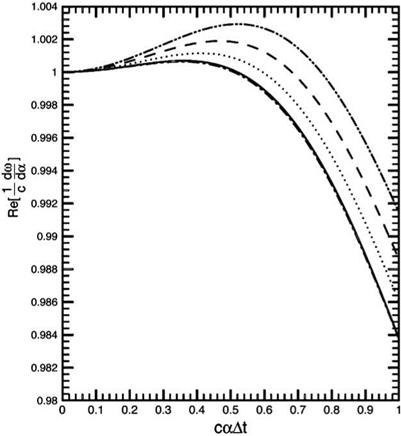
Since dm/da is not a constant equal to c even if da/da = 1.0, numerical dispersion is introduced by the use of the Runge-Kutta scheme. A plot of Re(dm/da) as a function of caAt (a = a assumed) for the low-dissipation low-dispersion Runge – Kutta (LDDRK) scheme is given as one of the curves in Figure 4.5. Notice that the group velocity drops below c for caAt > 0.5. The group velocity is less than the exact wave speed by at least 0.2 percent for caAt > 0.65. Waves in this range will form trailing waves.

To illustrate numerical dispersion due to temporal discretization, consider com­puting the solution of Eq. (4.11) with initial condition,

using the 15-point stencil DRP scheme for spatial discretization and the standard fourth-order Runge-Kutta scheme for temporal discretization. For convenience, the wave speed c is set equal to unity. The computed results are shown in Figure 4.4. Figure 4.4a shows the computed waveform after the pulse has propagated a distance of 608 mesh spacings using a very small time step At = 0.25Ax. The computed result is indistinguishable from the exact solution. Figure 4.4b shows the computed result when a larger At, At = 0.76Ax, is used. There is no question that the pulse is slightly dispersed. The cause is temporal discretization. For comparison purposes, Figure 4.4c shows the computed waveform using the LDDRK scheme of Hu et al. (1996) with At = 0.76Ax. There is definitely an improvement with the use of this scheme. However, there are still some trailing waves, a manifestation of numerical dispersion. For the initial condition (4.31), a small fraction of the initial pulse has

a wave number larger than a Ax = 0.855 corresponding to a At = 0.65. This part of the initial spectrum will propagate slower according to the group velocity curve of Figure 4.5. They show up as trailing waves. Finally, Figure 4.4d shows the computed result of the four-level time marching DRP scheme. The four-level scheme computes the derivative function once per step. The single step Runge-Kutta scheme computes the derivative function four times per step. Thus, to compare the results based on nearly the same workload, the time step of the DRP scheme is taken to be a quarter of that of the Runge-Kutta scheme, i. e., At = 0.19Ax. As can be seen, the results of Figures 4.4b, 4.4c, and 4.4d seem to indicate that the DRP scheme has less dispersion due to temporal discretization.

For certain wave propagation problems, minimizing dispersion error could be an important consideration. To do so, one might choose the free parameters or constants of the Runge-Kutta scheme to minimize the difference between the group velocity and the exact velocity of propagation of the governing wave equation. For the simple convective wave equation, the group velocity is given by Eq. (4.30). Suppose in (4.28) c1 and c2 are given the values of 1.0 and 0.5, but allow c3 and c4 to be free parameters. These parameters are then chosen to minimize the square of

the difference between the group velocity and the exact wave speed c = 1 over a band of wave number. It will be assumed that the spatial discretization is exact; i. e., a = a. Thus, c3 and c4 are chosen to minimize the integral,

Table 4.1 gives the values of c3 and c4 for different choices of n. The group velocity Re (dm/da) as a function of caAt corresponding to these choices of c3 and c4 is plotted in Figure 4.5. It is clear from this figure that by using a large n the minimization procedure forces a large band of wave number to have a group velocity closer to c. However, it is a feature of mean squared minimization that this also leads to a larger overshoot. So one might select a compromise between a larger bandwidth with a normalized group velocity closer to 1.0 and a smaller overshoot. Plotted also in Figure 4.5 is the group velocity curve of the LDDRK scheme. It turns out that it is almost identical to that of the choice n = 0.6. This is strictly a coincidence! But this appears to offer an explanation of why the LDDRK scheme does not incur excessive numerical dispersion error arising from temporal discretization.

Let us consider the solution of the simple convective wave equation:

d U d U

+ c = 0 dt dx

and initial condition
t = 0, u(x, 0) = Ф(х).
The Fourier-Laplace transform of (4.11) leads to , 4′ іФ (a) (a 1 (ш — ca) u=——- , (4.12) 2n where U is the Fourier-Laplace transform of u. Ф(a) is the Fourier transform of initial condition u(x, 0). Thus, U is given by
іФ (a) 2п (ш — ca)
(4.13)
The poles of Eq. (4.13) are found by setting the denominator to zero. This yields
ш = ca	(4.14)
which is the dispersion relation. The group velocity or wave speed is given by йш/da. In the case of Eq. (4.11), by using dispersion relation (4.14), the group velocity is
dш da
(4.15)
so that all wave components propagate with the same speed. That is to say, the waves supported by the convective wave equation are nondispersive. Now Eq. (4.11) may be fully discretized by first rewriting it as a system of two equations, each involving only either a temporal or spatial derivative, as follows:
This set of finite difference equations (Eq. 4.16) with discrete variables I and n may be generalized into a set of finite difference equations with continuous variables x

and t. They are as follows:

N

K(x, t) =——– ^2 ajU(x + jAx, t) (4.17a)

AX j=-N

3

u(x, t + At) = u(x, t) + At ^2 bjK(x, t — jAt), (4.17b)

j=0

with initial condition

( Ф(x), 0 < t < At

u(x, t) = (4.17c)

I 0, t < 0.

By taking the Fourier-Laplace transform of problem (4.17) and using the Shifting Theorem (see Appendix A), it is straightforward to find, after some algebra, that the solution is

ІФ (a)

2п (ш — ca)

where U is the Fourier-Laplace transform of the solution of the finite difference equation (4.17). Eq. (4.18) is identical to the Fourier-Laplace transform of the solu­tion of the original convective wave equation; i. e., Eq. (4.13), if ш and a in Eq. (4.18) are replaced by ш and a.

The exact solution of the finite difference solution of (4.11) is given by the inverse transform of Eq. (4.18) as follows:

The double integral may be evaluated by first calculating the contributions of the poles in the ш plane. The poles are given by the zeros of the denominator of the integrand, that is, the roots of

ш(ш) = ca(a). (4.20)

Eq. (4.20) is the dispersion relation. This is formally the same as the dispersion relation of the original partial differential equation; i. e., Eq. (4.14), provided ш is replaced by ш and a is replaced by a. For this reason, the finite difference scheme is referred to as dispersion-relation-preserving (DRP).

For a four-level time marching scheme, there would be four poles or Eq. (4.20) has four roots. Let the poles be ш = шj (a), j = 1, 2, 3, 4. One of the poles has Im(«) nearly equal to zero. This is the pole that corresponds to the physical solution. The other poles lead to solutions that are heavily damped.

Numerical dispersion can arise from spatial as well as temporal discretization. Numerical dispersion due to spatial discretization alone will be considered first. For this purpose, the limit At ^ 0 is applied, that is, time is treated exactly. This is

The integrand has a pole at ш = ca(a). On deforming the inverse contour Г to pick up this pole in the ш plane, it is easy to find through the use of the Residue Theorem

TO

u(x, t) = J Ф(a)ei(ax —ш) da. (4.23)

— то ш=са( a)

Now for large t (with x/t fixed), the a-integral of Eq. (4.23) may be evaluated by the method of stationary phase (see Appendix A). The stationary phase point a = as is given by the zero of the derivative of the phase function Ф = (ax/t — ca(a)) with respect to a. This leads to

which yields as as a function of x/t. The asymptotic solution is

where sgn(z) is the sign of z.

Now, ш and a are related by Eq. (4.22). In general, da/da is not a constant equal to 1, so that the group velocity varies with wave number. Different wave numbers of the initial disturbances will propagate with a slightly different speed leading to numerical dispersion.

In the more general case of solution (4.19), when both spatial and temporal dis­cretization are used, the group velocity may be calculated by implicit differentiation of Eq. (4.20). This gives

da

dm = C da da dm

dш

Eq. (4.26) indicates that numerical dispersion can be the result of imperfect spatial discretization, i. e., da/da = 1, or imperfect temporal discretization, i. e., drn/drn = 1. Consideration of imperfect time discretization will be deferred to later because it is quite involved. The effect of dispersion due to spatial discretization will now be illustrated by a numerical example.

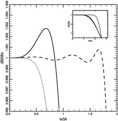
For the convective wave equation (4.11), Eq. (4.24) reveals that the variation in group velocity is caused by the variation of the slope of the a Ax versus a Ax curve. Figure 4.2 shows the da/da versus a Ax curves for the 7-point and 15-point

stencil DRP finite difference schemes. Notice that the da/da curve for the 7-point stencil DRP scheme has a peak at a Ax = 0.67 at which da/da = 1.00276. That is, the wave component with a Ax = 0.67 (wave with 9.38 mesh points per wavelength) will propagate faster than the exact wave speed da/da = 1.0 by about 0.3 percent. Suppose, in a computation, the waves propagate over a distance of 400 mesh points. In this case, when the main part of the wave packet reaches x = 400, the wave com­ponent with a Ax = 0.67 will reach x = 401.1. Under these circumstances, numerical dispersion would just be noticeable as wave dispersion exceeds one mesh point. On the other hand, if the standard sixth-order scheme is used instead, severe numerical dispersion will result when the main wave reaches x = 400. Waves in the wave num­ber range of a Ax > 0.6, having a group velocity less than 1.0, would form trailing waves.

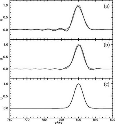
A relevant question to ask is how to reduce numerical dispersion due to spatial discretization. This can be done by using a scheme with a larger stencil. Figure 4.2 shows the da/da curve for the 15-point stencil DRP scheme. For aAx < 1.73, the group velocity differs from 1.0 by no more than 0.1 percent. Thus, if the wave packet of the solution contains only waves with wave number aAx < 1.73, then there will be no observable numerical dispersion even after the wave packet propagates over a distance of up to 1000 mesh points. As a concrete example, Figure 4.3 shows the

computed solution of the convective wave equation (4.11) with initial condition in the form of a Gaussian with a half-width of 3 mesh spacings,

u(x, 0) = e-(ln2)()2,

using the standard sixth-order scheme, the 7-point stencil, and the 15-point stencil DRP scheme. It is easy to see that there is significant numerical dispersion (with extensive trailing waves) when computed by the standard sixth-order scheme. The 7-point stencil DRP scheme is better. Both schemes, having the same stencil size, require the same amount of computation. The solution by the 15-point stencil is even better. For all intents and purposes, the solution is identical numerically to the exact solution.

Note that by Eq. (4.8), for large t,

. da

a + [x — m (a)t—– > a

. da

—m + [x — m (a)t- > —m,

dt

where m'(a) = (dm/da). Thus, locally, вx and —вt (subscript denotes partial deriva­tive) may be taken as the wave number and angular frequency as t ^ to. To find the phase velocity, one may keep в constant in Eq. (4.8) and differentiate with respect to t to obtain

r da dx

[x — m (a)t ——+ a— m = 0.

d t dt

For large t, by the above equation, the phase velocity is found to be

Now the asymptotic solution (4.6)-(4.9) may be given the following interpretation.

1. Each Fourier component with wave number a is constant along a ray in the x-t plane and propagates with group velocity m'(a) as shown in Figure 4.1. This is because x = m'(a) t so that a is a constant along a given line (ray) x/t = constant.

Figure 4.1. (a) Rays of x = K(a)t for constant a in the x-t diagram. (b) Ini­tial energy spectrum.

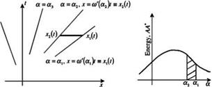Furthermore, dx/dt = K(a), suggesting that K(a), the group velocity, is the speed of propagation of wave number a.

2. Far away, the waves may be regarded as initiated locally near x = 0. After a period of time, the waves spread out in space because a different Fourier component with different wave number a propagates with different speed (O(a) = 0), see Figure 4.1a.

A quantity of interest in wave propagation is the wave energy that is A2 = AA* (* denotes the complex conjugate). The wave energy, Q(t), between two rays x = x1(t) = o'(a1) t and x = x2(t) = K(a2) t (see Figure 4.1a) is

With t fixed, a change of integration variable from x to a gives

dx = t O’ (a)da.

Hence,

H(a, K) dD do

Q(t)

Therefore, energy is constant between group lines. In other words, the wave energy of the initial energy spectrum (Figure 4.1b) propagates with group velocity. The group lines diverge with a separation that increases with t. Hence, the wave amplitude A decreases as t-(1/2).

It is important to point out that this analysis clearly shows that propagation speed and dispersion have nothing to do with phase velocity. Dispersion arises because of the variation of group velocity with wave number. For a more detailed treatment of dispersive waves, a reading of the book by Whitham (1974) is highly recommended.

Many physical systems support dispersive waves. Examples of commonly encoun­tered dispersive waves are small-amplitude water waves, waves in stratified fluid, elastic waves, and magnetohydrodynamic waves. A common feature of these dis­persive waves is that they are governed by linear partial differential equations with constant coefficients. The following are some of these equations.

a.

Klein-Gordon equation

b. Beam equation

д2ф + 2 д4ф = 0 W + p 9X4 = °-

c. Linearized Korteweg de Vries equation for water waves

дф д 3ф

~dt + p~X “ 0

d. Linearized Boussinesq equation for water and elastic waves

Э2ф _ 2 дф _ 2 д4ф = 0 dt2 а дх2 ^ дХ2дt2

Because these equations are linear with constant coefficients, they can be read­ily solved by Fourier-Laplace transform. The Fourier-Laplace transforms of these equations are

(a) (of2 _ (fa2 _ p2)ф = H1 (а, ш).

(b) (of2 _ p2a4)ф = H2(а, ш).

(c) (ш + pa3)ф = H3(a).

(d) (ш2 _ (fa2 + p2a2of2)ф = H4(а, ш).

The right-hand side of each of these equations represents some arbitrary initial conditions. The bracket multiplying the transform of the unknown on the left side of each equation is called the dispersion function, which will be denoted by D(a, m). The dispersion relation of the dispersive waves is given by the zeros of the dispersion function; i. e.,

D(a, m) = 0 ^ ш = ш(а).

Eq. (4.1) is a relationship between wave number a and angular frequency ш.

The solution of a dispersive wave system in wave number space, in general, may be written in the following form:

H(а, ш)

и =————-

D(a, ш)

The corresponding solution in physical space is found by inverting the transforms of Eq. (4.2) as follows:

и(х, t)	(4.3)

Suppose, for real a, the dispersion relation has a simple real zero. That is, ш(а) is a solution of

D(a, ш(а)) = 0.

Thus, for the ш-integral of Eq. (4.3), there is a pole lying on real ш-axis. The contribu­tion of this pole can be found by evaluating the ш-integral by the Residue Theorem. This gives, t > 0

и(х, t)

where Ф = a(x/t) — m(a) is the phase function of the integral. For large t, Eq. (4.5) may be evaluated asymptotically by the method of stationary phase (see Appendix B). The stationary phase point as is given by

Subscript s indicates the evaluation at a = as(x/t). In the following, the subscript s is dropped with the understanding that a is as(x/t) and m is m(as). The asymptotic formula may be rewritten in the compact form as follows:

Acoustics are governed by the compressible Navier-Stokes equations. In most cases, molecular viscosity is unimportant, so that the use of Euler equations is sufficient. In solving the Navier-Stokes or Euler equations computationally, the first step is to perform a discretized approximation to the spatial and temporal derivatives. This converts the partial differential equations to a set of partial difference equations. However, one must recognize that the solutions of the discretized equations are not the same as those of the original partial differential equations. A central effort of computational aeroacoustics (CAA) is to understand mathematically the behavior of the solution of the discretized equations and to quantify and minimize the error. Here, error is referred to as the difference between the solution of the original partial differential equations and the partial difference system.

Invariably, finite difference approximation of the governing equations of acous­tics will result in a dispersive wave system (Vichnevetsky and Bowles, 1982; Tre – fethen, 1982; Tam and Webb, 1993; Tam 1995), even though the waves supported by the original partial differential equations are nondispersive. This is an extremely important point and should be clearly understood by all CAA investigators and users.

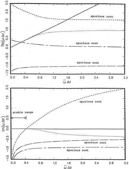
It is easily seen from Eq. (3.16) that the relationship between rnAt and rnAt is not one to one. This means that there are spurious numerical solutions. These spurious solutions could cause numerical instability, so it is necessary to find out about their characteristics.

Eq. (3.16) may be rewritten in the form as follows:

^ ^ + V2 + (b0 + =At)z – = 0. (3.20)

where z = elmAt. Thus, given a «At, there are four roots of elmA. In other words, there are four values of «At that would give the same «At when substituted into Eq. (3.16). For the values of bj (j = 0, 1, 2, 3) given by formula (3.19), the val­ues of the four roots of «At as functions of «At have been found. The real and imaginary part of these roots over the range 0 < «At < n are plotted in Fig­ure 3.1. In the range «At < 0.41, the imaginary parts of all the four roots are neg­ative. Recall that the solution «, given by the inverse transform of Eq. (3.11), is a superposition of elemental solutions having time dependence of the form e-lmt. If Im(«) is negative, the solution is damped in time. However, for «At > 0.41,

one spurious root has a positive imaginary part. The solution corresponding to this root will grow, in time overwhelming the physical solution, and lead to numerical instability.

On examining the real parts of the four roots, it is seen that one of the roots gives mAt = mAt over the range mAt < 0.41. This is the physical root. The others are spurious. The physical root has a very small imaginary part up to mAt = 0.41. That is, there is very little numerical damping. A more detailed investigation reveals that, for this root, Im (mAt) = -0.118 x 10-4 for mAt = 0.19. This is reasonably small. It is recommended that At be chosen such that mAt < 0.19. This would automatically guarantee numerical stability and negligible numerical damping.

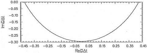
In most wave propagation problems, to be discussed later, mAt is real. In this case, this stability consideration is sufficient. However, if the wave is damped by some physical process, or artificial damping is added to the computation scheme for the purpose of removing spurious waves from the numerical solution, then mAt is complex. To include this more general case, it is necessary to consider the four solutions of Eq. (3.20) for mAt in the complex plane. It is straightforward to find that the stable region (all the four roots of mAt have a negative imaginary part) is confined to a small nearly semicircular region in the lower mAt plane. This is shown in Figure 3.2. This stability diagram plays an important role in the choice of time step At in time marching computation. Numerical stability will be discussed in Chapter 5.

EXERCISES 3.1. Construct an optimized two-level time marching scheme for the differential equation

F (u).

Find the stability region in the complex mAt plane. 3.2. Consider the solution of the initial value problem

by finite difference approximation. Let the spatial derivative be approximated by a second-order central difference equation. The convective wave equation becomes

dul c

~dt _- 2^(Ul+1 – Ul-1 X

where l is the spatial index. Difference-differential equation (C) may be integrated by the four-level optimized time marching scheme. On writing out in full, the finite difference equations are

Consider a Fourier-Laplace transform component of the solution

U^n’) __ Ае^(1аДх— n^At)

Perform a Von Neumann stability analysis of the finite difference scheme by sub­stituting Eq. (F) into (D) and (E). Show that this yields the dispersion relation as follows:

ш(ш) _ ca(a),

where a is the stencil wave number of the second-order central difference scheme and ш is the angular frequency of the four-level time marching scheme.

(a) Show that the scheme is stable if

0. 41 Дх

At <————

c

(b) Implement the time marching scheme on a computer. Take At to be slightly larger than that given by Eq. (H). Compute the solution in time up to t _ 400 with (B) as the initial condition to see whether the solution is unstable (i. e., grows exponentially in time).

(c) Verify computationally that, if At is chosen according to condition (H), the numerical scheme is stable. Furthermore, if At is taken to be less than or equal to 0.19 Дх/c, an excellent numerical solution can be obtained.

Suppose u(t) is the solution of Eq. (3.1). In a multilevel time discretization method, the time axis is divided into a uniform grid with time step At. It will be assumed that the values of u and du/dt are known at time level n, n – 1, n – 2, n – 3. (Note: In CAA, du/dt is given by the governing equations of motion.) To advance to the next time level, the following four-level finite difference approximation is used:

(3.9)

The last term on the right side of Eq. (3.9) may be regarded as a weighted average of the time derivatives at the last 4 mesh points. There are four constants, namely, b0, b1, b2, and b3, that are to be selected. To ensure that the scheme is consistent, it is suggested to choose three of the four coefficients, say bj (j = 1, 2, 3), so that when the terms in Eq. (3.9) are expanded in a Taylor series in At they match to the order (At)2. This leaves one free parameter, b0. The relation between the other coefficients and b0 are as follows:

ro – i s’ лп

b1 =-3b0 + 12 ’ b2 = 3b0 3, b3 =-b0 + 12. (3.10)

The remaining coefficient b0 will now be determined by requiring the Laplace trans­form of the finite difference scheme (3.9) to be a good approximation of that of the partial derivative.

The Laplace transform and its inverse of a function f(t) are related by (see Appendix A) the following:

(Ю

f(m) = 2П j f (t)elmtdt, f (t) = j f(a)e~imtda. (3.11)

0 г

The inverse contour Г is a line in the upper half m plane parallel to the real m­axis above all poles and singularities. Before Laplace transform can be applied to Eq. (3.9), it is necessary to generalize the equation to one with a continuous variable. This can easily be done. The result is as follows:

3

^ du(t – jAt) ,„„„4

u(t + At) = u(t) + At bj—————– . (3.12)

d t

Eq. (3.12) reduces to Eq. (3.9) by setting t = nAt. It will be assumed, for the time being, that u(t) satisfies the following trivial initial conditions (the case with general initial conditions will be discussed later); i. e.,

In Appendix A, the following shifting theorem for Laplace transform is proven:

Transform of f (t + A) = e-imAf; ~ = Laplace transform (3.14)

On applying the shifting theorem to Eq. (3.12), it is easy to find

Thus,

.i(e~mAt -1) _ ( f tdU

– i——————– u = transform of — . (3.15)

3 ,. a V d t f

AtJ2 bjeijmAt

j=0

The Laplace transform of the time derivative of u is – i’«U. Thus, by comparing the two sides of Eq. (3.15), the quantity

i(e-iaAt – 1)

3

At ^2 b. eijmAt
j=0 j

is the effective angular frequency of the time marching scheme (3.9). The weighted error Ex incurred by using ш to approximate ш will be defined as

z

E1 = j [a[Re(«At – rnAt)]2 + (1 – a)[Im(«At – rnAt)]2}d(«At), (3.17)

-z

where Re() and Im() are the real and imaginary part of (). a is the weight and z is the frequency range. One expects ш to be a good approximation of ш. On substituting ш from Eqs. (3.16) and (3.10) into Eq. (3.17), Ex becomes a function of b0 alone. b0 will be chosen so that Ex is a minimum. Therefore, b0 is given by the root of

A range of possible values of a and z has been used in Eq. (3.18) to determine b0 and, hence, b1, b2, and b3. After considering the effect on the range of useful frequency and numerical damping rate, the values a = 0.36 and z = 0.5 were selected. For this value of a and z, the values of the coefficients bj (j = 0,1,2,3) are

b0 = 2.3025580888383, b1 = -2.4910075998482 b2 = 1.5743409331815, b3 = -0.3858914221716.

One of the most popular time marching methods is the Runge-Kutta (RK) scheme. The RK scheme is based on Taylor series truncation. A widely used RK scheme is the fourth-order method. To illustrate the basic approach of the RK method, let the time axis be divided into increments of At. Suppose the solution of a differential equation,

£=f<">- (31)

where u and F are vectors, and time level n is known. To find the solution at the next time level (n + 1), four evaluations of the derivative function F are performed (fourth-order RK). These intermediate evaluations provide indirectly the high-order derivatives of u so that a matching of high-order terms in At in a Taylor series expansion becomes possible. The following is a very general form of the fourth- order RK scheme:

4

u(n+1) = u(n) + J2 wjКj j=1

К = F (uw) At k2 = F (uw + p2k1) At k3 = F (u(n) + e3k2) At k4 = F (u(n) + e4k3) At.

Superscript (n) indicates the time level. The constants в2, в3, в4, w1, w2, w3, and w4 are chosen so that, when the left and right sides of Eq. (3.2) are expanded in Taylor series for small At, they are matched to order (At)4. For the standard fourth-order scheme, the constants are assigned the following values:

1 11

в2 = в3 = 2 ’ в4 = 1-0, w1 = w4 = 6 ’ w2 = w3 = 3 • (3.3)

It is known that this choice is not unique. Other choices are possible within the requirement that the Taylor series expansions of Eq. (3.2) are matched to terms of order (At)4. An alternative choice proposed by Hu et al. (1996) called the low – dissipation low-dispersion Runge-Kutta (LDDRK) scheme is widely used in com­putational aeroacoustics (CAA). In formulating the LDDRK scheme, attention is focused on discretizing the time derivative of the convective wave equation,

d u d u

—– + c— = 0,

dt dx

rather than Eq. (3.1). Suppose the spatial derivative of Eq. (3.4) is approximated by a high-order finite difference scheme. The Fourier transform of the finite difference equation is

du __ — = – icau, dt

where u is the Fourier transform of u and a(a) is the wave number of the spatial finite difference approximation of 9/dx.

Now, if the fourth-order RK scheme (3.2) is applied to Eq. (3.5), it is easy to find, after some algebra, that the time marching scheme becomes

(3.7)

It is a simple matter to show that, for the standard fourth-order RK scheme, Cj = jp
According to LDDRK, the cj constants are assigned the following values:

c1 = 1.0, c2 = 0.5, c3 = 0.162997, c4 = 0.0407574. (3.8)

This choice is motivated by numerical stability consideration and the desire to use the largest At permissible. It turns out that the choice also keeps the numerical dispersion low, as pointed out by Tam (2004). That LDDRK is a low dispersion scheme will be discussed in the next chapter.

To implement the LDDRK scheme, it is necessary to find a set of numerical values of вj and wjs when the cjs are given by Eq. (3.8). A simple way to keep the scheme close to the standard fourth-order scheme is to keep the values of в;- the same as the standard scheme and to determine the values of Wj by solving Eq. (3.7) as a linear system of equations. The values of wj’s are as follows:

W1 = w4 = 0.1630296, w2 = 0.348012, w3 = 0.3259288.