Category FLIGHT MECHANICS MODELING and ANALYSIS

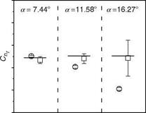
An unstable aircraft cannot fly without the aid of a flight controller, thereby render­ing the entire system as a closed loop control system. However, the estimation of derivatives of basic unstable aircraft (open loop system) is of primary interest for many applications in the field of flight mechanics, especially for the validation of the math models used for control-law design. The accuracy of the estimated derivatives in such cases is adversely affected by the feedback from the flight controller, which tends to produce highly damped responses and correlated I/O variables. Using the filter error program it was shown that better estimation can be achieved if modeling errors arising from data correlation are treated as process noise. Parameter estimation of an augmented aircraft equipped with a controller was carried out using output error and FEMs. It was shown that the feedback signals from the controller and the aileron-rudder interconnect operation cause correlations between the I/O variables, which degrade the accuracy of the parameter estimates. FEM was found to yield reliable parameter estimates, while the aircraft derivatives estimated from OEM did not compare well with the reference derivative values. Parameter-estimation results from data generated from a research simulator for an unstable augmented aircraft are plotted in Figure 9.4. Due to the model compensation ability of FEM, the derivatives estimated show better match with wind-tunnel values compared to the derivatives estimated from OEM [17].

9.4.2 Basic and Modified Transport Aircraft

A program to modify a transport aircraft to carry some electronics payloads was taken up. It was important to establish the incremental effects on the dynamic

FIGURE 9.4 Parameter estimation using FEM and OEM for an unstable/augmented aircraft FA2.

derivatives due to the modification in the aircraft. The aircraft has a medium range with two Rolls Royce Dart turboprop engines. It has manually operated controls for elevators, rudder, and starboard ailerons. On the modified aircraft an external structure was mounted on the pair of pylons fixed to the fuselage of the basic aircraft. The modified aircraft was expected to have some altered characteristics compared to the basic aircraft. Hence, it was very important to predict its characteristics and handling qualities. Several planned maneuvers were performed on this transport aircraft: DR, steady turn, sideslip wings level, sideslip steady heading, roll perform­ance, longitudinal stability, SP/phugoid, stall, and RC. The dynamic data were acquired at the rate of 32 samples/s and corrected using kinematic consistency checking and subsequently used for parameter estimation. The math models used are given in Ref. [18]. Some results are shown in Table 9.4. The other results were found to be consistent across various flight conditions (Mach number and altitude).

Some LD characteristics of the modified aircraft are given in Table 9.5. The damping-in-roll and the static stability of the modified aircraft were quite improved compared to the basic aircraft. However, the DR frequency and damping were poor for the former when compared to the latter. The LD static stability was improved; this could be due to the pylons providing additional vertical surface above the fuselage (similar to the vertical tail). The predicted longitudinal and LD HQs were validated by the flight (test data) derived HQs for both the aircraft [18].

A new procedure for estimation of neutral point (Appendix A) is applied to the basic and the modified configurations [19]. The experiments were conducted at three CG points. In the classical method of neutral point estimation, the lift coefficient was determined from the airspeed and the weight data. The results (on the average) of neutral and maneuver points (as percentage of MAC) estimated by using parameter – estimation method are also shown in Table 9.4. The new method is expected to be highly reliable because the data used are corrected by kinematic consistency, and the longitudinal static and maneuver stability of the aircraft are extracted from the

SP dynamic response parameters Ma and the natural frequency ы^, which vary consistently with the location of CG. We see that the static stability of the modified aircraft is reduced compared to the basic aircraft; however, the damping is increased as seen in Table 9.4.

This is a modern high-performance fighter aircraft fully instrumented for the SIPE experiments. The maneuvers conducted were short period (SP), lateral-directional (LD), roller coaster (RC), slowdown (SD), and wind-up turn (WUT). The latter three maneuvers are dynamic maneuvers for determination of drag polars from the flight test data using parameter-estimation methods. The idea behind this is that these maneuvers save flight test time compared to the steady-state methods (Chapter 7). The RC maneuver data were generated for Mach range 0.6-0.8 for 1g excursion of acceleration covering 0°-9° AOA. The SD maneuver is a low-speed maneuver at about 0.4 Mach and the AOA range covered is 9°-19°. The WUT involves a Mach range 0.6-0.8 steep turn of decreasing radius with “g” force varying from 1g to 8g. The AOA range is 8°-19°. The WUT is a combined longitudinal/lateral maneuver. The various tests were performed at 1.5, 3, and 6 km altitudes. The signals were sampled at 16/32 samples/s. Where applicable the sideslip angle correction factors with respect to altitude and Mach were used. Various math models used for the data analysis are given in Ref. [16]. Thrust data were used as input to the mathematical model. For drag polar estimation, the model-based approach was used as against the static/steady-state approach, since dynamic maneuvers were performed. This shifts the burden from flying aircraft at several AOA/Mach numbers (to obtain the static

stability and control derivatives as well as drag polars (by estimating lift and drag coefficients as a function Mach number/AOA) from the dynamic maneuvers (RC, SD, and WUT). Most of the (longitudinal and LD) flight determined derivatives (FDDs) as well as the drag polars compared well with the manufacturer’s data. The flight-determined longitudinal HQ met the Level 1 requirements. The flight-determined SP natural frequency varied from 2.3 to 3.65 rad/s and the damping ratio was 0.3. The Dutch roll (DR) frequency was determined as 2.5 to 3.4 rad/s. The neutral point was also determined from the real flight data and the results are shown in Table 9.3.

intention of estimation of stability and control derivatives and performance charac­teristics. To the extent possible, the experiments were conducted very carefully, data were gathered with adequate sampling rates, and where necessary data compatibility analysis was carried out and the corrected data were used for parameter estimation. In a few cases, the data generated from the flight simulator have been used. For the sake of brevity Cramer-Rao uncertainty bounds are not given and the aerodynamic derivatives are based on only a few data sets, where the repeat runs are not available, due to cost and time constraints in conducting several flight tests. Despite this, the results are found to be reasonably good and are representative of the characteristics of the specified aircraft or vehicle. Since most of the data analyzed for these case studies are real flight data, it gives a good feel and experience of the application of flight data analysis procedures and parameter-estimation methods. Wherever applic­able the multiple maneuver analysis and model validation were carried out. Often the aerodynamic derivatives are obtained as a function of AOA or Mach number. The plots of these derivatives with respect to these independent parameters would be very useful. These plots would depict the trends, linear or nonlinear, and thus, reveal the specific characteristic variation of the derivatives. Also, it would be a good practice to plot these derivatives with respect to say AOA, such that any graphical difference in the variation or any discerning effects during comparison of the values with other derivatives show the correct correlations in the percentage differences and the graphical distances of these variations. For this purpose, the minimum and maximum values of all derivatives are determined and then the y-axis scale is chosen by multiplying these extreme values with the same factor, say 1.5. This factor remains the same for all the derivatives. With this method, any graphical difference (meas­ured in a distance unit) in any derivative will correspond to the same percentage difference in the numerical values.

There are two major approaches in SOEMs. In the equation decoupling method (EDM), the system state matrix is decoupled (1) only diagonal elements pertaining to each of the integrated states, supposed to be the stable part and (2) the off-diagonal elements associated with the measured states. Thus, the state equations are decoupled and the unstable system is changed to a stable one. The stabilization of OEM by means of measured states would prevent the divergence of the integrated states. The measured states are used and the input vector u is augmented with the measured states xm to give

The integrated stable variables are present only in the Ad part, and all the off-diagonal variables have measured states. This renders each differential equation to be inte­grated independently of the others.

In the regression analysis SOEM, the measured states are used with those param­eters in the state matrix that are responsible for instability in the system and integrated states are used with the remaining parameters. Matrix A is put into two parts: (1) one containing parameters that do not contribute to instability and (2) the other with parameters that contribute to system instability. The partitioned system has the form

The integrated states are used for the stable part of the system matrix and the measured states for the parameters contributing to the unstable part of the system.

Thus, stabilized OEMs seem to fall in between EEMs that use the measured states and OEMs and can be said to belong to a class of mixed equation error-OEMs. OEM does not work directly for unstable systems because numerical integration of the system equations causes divergence. For SOEMs, since the measured states (obtained from the unstable system operating in closed loop) are stable, their use in the estimation process attempts to prevent the divergence. The parameter estima­tion of a basic unstable system directly in a manner similar to that of OEM for a stable plant is accomplished and this is established by the asymptotic analysis of SOEMs when applied to unstable systems [1].

In certain practical applications, it is required to estimate the parameters of the open loop system (which might be inherently unstable) from the data generated when the system is operating in a closed loop. The feedback causes correlations between the input and output variables and identifiability problems. In the augmented system, the measured responses would not display the modes of the system adequately as the feedback is generating controlled responses. The complexity of the estimation problem is more when the basic system is unstable because the integration of the state model could lead to numerical divergence and the measured data would be usually corrupted by process and measurement noises. The EEM does not involve direct integration of the system’s equations and hence can be used for parameter estimation of such unstable systems. The EKF-UD approaches can be used for parameter estimation of unstable systems because of the inherent stabilization properties of the filters [1]. OEM poses some difficulties when applied to highly unstable systems since the numerical integration of the unstable state model equa­tions would lead to divergence. One can provide artificial stabilization in the model (in the software algorithm) used for parameter estimation resulting in the feedback – in-model method. This requires good engineering judgment. Another way to cir­cumvent this problem is to use measured states in the estimation, leading to the stabilized output error method (SOEM) [1]. The FEM is the most general approach to the problem of parameter estimation. FEM treats the errors arising from data

correlation as process noise, which is suitably accounted for by the KF part of FEM. A detailed exposition of FEM is given in Refs. [1,5].

Many real-life dynamic systems are nonlinear and the estimation of states of such systems is often required. The nonlinear system can be expressed as

variables at time t = 0, bu represents the bias parameters in control inputs, by represents the biases in model responses y, and b represents the parameters in the mathematical model of the system. One needs to linearize the nonlinear functions f and h and apply the KF with proper modifications to these linearized models. The linearizations will be around previous/current best state estimates that are more likely to represent the truth. Simultaneous estimation of states and parameters is achieved by augmenting the state vector with unknown parameters, as additional states, and then using the filtering algorithm with the augmented system nonlinear model. The new augmented state vector is given as

We notice the time-varying nature of A, H, and f because they are evaluated at current state estimate, which varies with time k.

Time Propagation

The states are propagated from the present state to the next time instant. The predicted state is given by

tk+1

The covariance matrix for state error propagates from instant k to k + 1 as

P(k + 1) = f(k)P(k)fT (k) + Ga (k)QGT (k) (9.59)

Measurement Update

The EKF updates the predicted estimates by incorporating the new measurements as follows:

xa(k + 1) = ~a(k + 1) + K(k + 1){Zm(k + 1) – ha[~a(k + 1), u(k + 1), t]} (9.60)

The covariance matrix is updated using the Kalman gain and the linearized meas­urement matrix. The Kalman gain is given by

K(k + 1) = P(k + 1)HT (k + 1)[H(k + 1)P(k + 1)HT (k + 1) + R]-1 (9.61)

The posteriori covariance matrix is given as

P(k + 1) = [/ – K(k + 1)H(k + 1)]P(k + 1) (9.62)

A sophisticated filter error method (FEM) accounts for process and measurement noise using a KF in the structure of the maximum likelihood/OEM (MLOEM). The details of this method are given in Ref. [1].

Kalman filtering has evolved to a very high state-of-the-art method for recursive state estimation of dynamic systems [14]. It has generated worldwide extensive applications to aerospace system and target tracking problems. It has an intuitively appealing state-space formulation and it gives algorithms that can be easily imple­mented on digital computers, since the filter is essentially a numerical algorithm and is the optimal state observer for the linear systems.

Being a model-based approach, it uses the system’s model in the filter:

x(k + 1) — fx(k) + Bu(k) + Gw(k) z(k) — Hx(k) + v(k)

The process noise w is a white Gaussian sequence with zero mean and covariance matrix Q, the measurement noise v is a white Gaussian noise sequence with zero mean and covariance matrix R, and f is the n x n transition matrix that propagates the states from k to k + 1. Given the mathematical model of the dynamic system, statistics Q and R of the noise processes, the noisy measurement data, and the input, the Kalman filter (KF) obtains the optimal estimate of the state, x, of the system. It is assumed that the values of the elements of f, B, and H are known.

Intuitively, the idea is to incorporate the measurement into the data-filtering process and obtain a refined estimate of the state. The algorithm is given as follows:

State/Covariance Evolution or Propagation

x(k + 1) = fx(k) (9.40)

P(k + 1) = fP(k)fT + GQGT (9.41)

Measurement Data/Covariance Filtering/Update

r(k + 1) = z(k + 1) – H~x(k + 1) (9.42)

K = PHT (HPHT + R)-1 (9.43)

x(k + 1) = x(k + 1) + Kr(k + 1) (9.44)

P = (I – KH)P (9.45)

The matrix S = HpHT + R is the covariance matrix of the residuals/innovations. The actual residuals can be computed from Equation 9.42 and these can be compared with standard deviations obtained by taking the square root of the diagonal elements of S. The performance of the filter can be evaluated by (1) checking the whiteness of the residuals and (2) comparing the computed covariance with the theoretical covariance obtained from the covariance equations of the filter. The test signifies that (1) the residuals being white, no information is left out to be utilized in the filter and (2) the computed covariance from the data matches the filter predictions/ theoretical estimates of the covariance. Thus, a proper tuning has been achieved. The KF could diverge due to many reasons [15]: (1) modeling errors due to the use of a highly approximated model of the nonlinear system; (2) choice of incorrect a priori statistics (P, Q, R); and (3) finite word length computation. For (3) a factorization-based filtering method should be used, or the filter should be imple­mented on a computer with large word length.

Let a linear dynamical system be described as

In many applications, the actual systems are of continuous time, but the measure­ments would be at discrete samples, with

E{v(k)} = 0; E{v(k)vT (l)} = R8kl (9.28)

We have the likelihood function as

The parameter vector b is obtained by maximizing the likelihood function with respect to b by minimizing the negative log likelihood function given as

L = – log p(zb, R)

1N

= 2 E [z(k) – y(k)]TR-1 [z(k) – y(k)] + N/2 log R + const (9.30)

2 k=1

The R can be estimated as

When the estimated value R is substituted in the likelihood function, the minimiza­tion of the cost function with respect to b results in

dL/db = – X (dy(b)/db)TR-1(z – y(b)) = 0 (9.32)

k

This set is a system of nonlinear equations and an iterative solution can be obtained by the quasi-linearization method, known as modified Newton-Raphson or Gauss-Newton method. We expand

y(b) = y(b + Db)

as

A version of the quasi-linearization is used for obtaining a workable solution for the OEM.

Substituting this approximation in Equation 9.34 we get

Ь new — Ь old + Dp

The CRB is a primary criterion for evaluating the accuracy of the estimated param­eters. MLE gives the measure of this parameter accuracy without any extra compu­tation. The information matrix is computed as

The diagonal elements of the inverse of the information matrix give the individual covariance, and the square roots of these elements are measures of the standard deviations called the CRBs. The OEM/MLE can also be applied to any nonlinear system. Computational and accuracy aspects are further discussed in Ref. [і].

9.3.2.2 produce the model responses which would closely match the measurements. A likelihood function, similar to a probability density function (PDF), is defined when measurements are used. This likelihood function is maximized to obtain the estimates of the parameters of the dynamic system. The OEM is an ML estimator, which accounts only for measurement noise and not process noise. The main idea is to define a function of the data and the unknown parameters. This function is called the likelihood function. The parameter estimates are those values that maximize this function. If bi, b2,…, br are the unknown parameters of a system and zi, z2,…, zn the measurements of the true values yi, y2,…, yn, then these true values could be made a function of these unknown parameters as

If z is a random variable with PDF p(z, b), then to estimate “b” from z, choose the value of b that maximizes the likelihood function L(z, b) = p(z, b). Thus, the problem of parameter estimation is reduced to maximization of a real function called the likelihood function (of the parameter b and the data z). In essence, “p” becomes “L” when the measurements are obtained and used in p. The parameter b, which makes this function most probable (to have yielded these measurements), is called the ML estimate. Such a likelihood function is given as

The main point in any estimator is to determine or predict the error made in the estimates relative to the true parameters, although the true parameters are unknown in the real sense. Only some statistical indicators for the errors can be worked out. The Cramer-Rao lower bound is, perhaps, the best measure for such errors. The likelihood function is defined as

L(z|b) = log p(z|b) (9.19)

The likelihood differential equation is obtained as

@ . p

—L(zjb) = L'(zjb) = j (zjb) = 0 (9.20)

The equation is nonlinear in b and a first-order approximation by Taylor’s series expansion is used to obtain /3:

The increment in b is obtained as

D8 = = -(L"(z/bo))_1L'(z/bo) (9.22)

L (zlbo)

The likelihood related partials can be evaluated when the details of the dynamic systems are specified. In a general sense, the expected value of the denominator of Equation 9.22 is defined as the information matrix:

Im(b) = E{-L’ ‘(zlb)} (9.23)

From Equation 9.23, we see that if there is large information content in the data, then |L"| tends to be large, and the uncertainty in estimate b is small (Equation 9.22). The Cramer-Rao inequality provides a lower bound to the variance of an unbiased estimator. If be(z) is any estimator of b based on the measurement z, and be(z) = E{be(z)}, the expectation of the estimate, then we have as the Cramer – Rao inequality, for unbiased estimator:

sbe > (Im(b))-1 (9.24)

For unbiased efficient estimator sb = I—1 (b). The inverse of the information matrix, for certain special cases, is the covariance matrix and hence we have the theoretical expression for the variance of the estimator. Thus, the actual variance in the estimator, for an efficient estimator, would be at least equal to the predicted variance, whereas for other cases it could be greater but not less than the predicted value. The predicted value provides the lower bound.

Several useful techniques are available in the literature for estimation of parameters [1] from flight data, the selection of which is governed by the complexity of the mathematical model, a priori knowledge about the system, and information on the noise characteristics in measured data. In general, the estimation technique provides the estimated values of the parameters along with their accuracies, in the form of standard errors or variances. In this section some widely used methods are briefly discussed.

9.3.2.1 Equation Error Method

In the equation error method (EEM), the measurements of the state variables and their derivatives are assumed to be available and used. The method is computation­ally simple and is a one-shot procedure. Since the measured states and their deriva­tives are used, the method would yield biased estimates, and hence it could be used as a start-up procedure for other methods. It minimizes a quadratic cost function of the error in the state equations to estimate the parameters. The EEM is applicable to linear as well as linear-in-parameter systems. The EEM can be applied to unstable systems because it does not involve any numerical integration of the system equa­tions that would otherwise cause divergence of certain state variables. Thus, the utilization of measured states and state-derivatives for estimation in the algorithm enables estimation of the parameters of unstable systems. If a system is described by the state equation

x = Ax + Bu; x(0) = X0

then the EE can be written as

e(k) xm Axm Bum (9 •11)

НСГС, Aa [A, xam

The cost function is given by

1 ^

J(b) 2 ‘У [Xm(k) Aaxam(k)] [Xm(k) Aaxam(k)]

2 k=1

and the estimator is given as

Example 9.1

The equation error formulation for parameter estimation of an aircraft is illustrated with one such state equation here. Let the moment equation be given

q = Maa + Mqq + MSt Se (9.15)

Then moment coefficients of Equation 9.15 are determined from the system of linear equations given by (Equation 9.15 is multiplied in turn by a, q, and Se)

^qa = M„5>2 + Mq^qa + MSt^ Sea ^qq = Ma^aq + Mq^q2 + Ms^^ Seq (9.16)

]T qSe = M^2 aSe + M^2 qSe + Ms^ S2e

Here, S is the summation over the data points (k = 1,…, N) of a, q, and Se signals. Combining the terms, we get

The above formulation can be expressed in a compact form as Y=Xp, and the equation error is formulated as e = Y — X/3 keeping in mind that there will be modeling and estimation errors combined in ‘‘e.’’ It is presumed that measurements of q, a, q, and Se are available. Then the equation error estimates of the parameters can be obtained using Equations 9.7 and 9.14.