Our heavyweight helicopter equal in the world does not have
In Rostov started production of the most load-lifting rotary-wing car The Russian holding «Helicopt[...]

Everything about aircrafts and helicopters. News and events in aviation worldwide. Civil, transportation, military helicopters and airplanes.

Everything about aircrafts and helicopters. News and events in aviation worldwide. Civil, transportation, military helicopters and airplanes.

Everything about aircrafts and helicopters. News and events in aviation worldwide. Civil, transportation, military helicopters and airplanes.

Everything about aircrafts and helicopters. News and events in aviation worldwide. Civil, transportation, military helicopters and airplanes.


Handling qualities criteria (HQC) depend on several factors [1]: type of aircraft, flight phase, and control system-aircraft characteristics. Airplanes are classified as
Class I: Small, light
Class II: Medium weight, low-to-medium maneuverability
Class III: Large, heavy, low-to-medium maneuverability
Class IV: High maneuverability
Flight operation phases are categorized as
Phase A: Nonterminal flight that requires rapid maneuvering, precision
tracking, or precise flight path control.
Phase B: Nonterminal flight that is normally accomplished using gradual,
moderate maneuvers and without precision tracking, although accurate flight path control may be required.
Phase C: Terminal flight that is normally accomplished using gradual man
euvers and usually requires accurate flight path control. This comprises takeoff, approach, and landing.
Flying qualities level of acceptability related to the ability to complete the mission are also predefined as
Level 1: Flying qualities clearly adequate for the flight phase of the mission.
Level 2: Flying qualities adequate to accomplish the mission flight phase, but
there would exist an increase in pilot workload or degradation in mission effectiveness, or both.
Level 3: Flying qualities such that the airplane can be controlled safely, but
pilot workload is excessive or mission effectiveness is inadequate or both are possible. Category flight phase A can be terminated safely and category flight phases B and C can be completed.
Primarily, the HQ criteria would be evaluated using mathematical models of the airplane as well as of the pilot/control systems. The quantitative requirements of the specifications are given in terms of parameters of a linear model of the aircraft. In the case of control system nonlinearities/HO response of the flight control-aircraft combination, an equivalent mathematical model would be defined. For all types of models the requirements in terms of frequency, damping ratio, and phase angles would apply. Some of these criteria are described next [6-26]. In fact Ref. [8] describes several HQC for fixed-wing aircraft and their rationale, algorithms (formulae, etc.), criteria requirements, and guide for application. However, Ref. [27] described an integrated handling qualities software (HQSW) package for rotorcraft and fixed-wing aircraft, with more emphasis on the former.
While flying and controlling an airplane, the human pilot must be using some strategy for flight operation. The human operator/pilot can be regarded as one of the controllers in the overall man-machine/aircraft interaction systems. In the pilot – aircraft system (PAS) to evaluate HQs, the human pilot’s mathematical model would play an important role. This math model describes the control behavior of the human pilot. Manual control tasks that a pilot is called upon to perform are compensatory, pursuit, precognitive, and preview. In a compensatory task only the system error is displayed or presented to the pilot. Precognitive task is one where the pilot experiences a pure open loop programmed control-like situation. One example is that the
overall input to the system is a sinusoidal, which is very quickly learned by the pilot who operates in precognitive mode.
10.3.1 Motion Plus Visual and Only Visual Cue Experiments
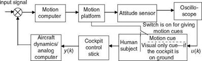
In manual control experiments with compensatory tracking tasks in a motion-based flight research simulator, a human operator’s control-theoretic mathematical models were obtained. The simulator facility had three degrees of freedom: pitch, roll, and heave motion [3,4]. The input-output data were generated while the operator performed a manual control task (Figure 10.2). Input to the pilot was in the form of a visual sensory stimulus as derived from the horizontal line on an oscilloscope, which represented a tracking error. The actual input signal was taken from the electrical signal equivalent to the display device. The tracking input was a band – limited random signal common to both the experiments. The output signal was derived from the movement of the stick used by the operator in performing the task. The idea was that first the operator performs the task while he or she is in the cockpit which was mounted on the moving base platform of the simulator. The tracking error was presented to the operator and he or she had to continuously try to keep the error at minimum. When the operator’s performance had reached a steady state, the data were recorded and subsequently sampled at 20 samples/s. The performance criterion was the integrated square error for the duration of the task. The human operator as a subject had to perform the same task repeatedly to reach his or her steady-state performance in terms of this criterion. Subsequently, for the same task the cockpit was unfastened from the moving base and placed on the ground and only visual cue was made available to the operator. However, since the motion platform will still be in action, its dynamics are common to both the experiments. Time-series/transfer function (TF) modeling was carried out for two such human operators while they independently tracked two types of dynamics simulated on an analog computer. Various model selection criteria were used and third-/fourth – order least squares (LS) time-series models in discrete-time domain (i. e., pulse TFs, 600 data points were used) were found adequate. Then, Bode diagrams were obtained from these pulse TFs and further analysis and interpretations were carried out. A human
|
Random
|
operator’s mathematical model (in the control-theoretic sense) in such a task can be defined by the LS model structure (Chapter 9):
A(q-l)y(k) = B(q-1)u(k) + e(k) (10.1)
As can be seen from Equation 10.1, the operator’s response naturally gets separated into the numerator and denominator contributions as [3]
![]() Hsp( jv) = B(jV)
Hsp( jv) = B(jV)
HEN( jv) = 1/A( jv)
Here, Hsp, the numerator part, is correlated to the human sensory and prediction part, and the denominator HEN to the equalizing and the neuromuscular parts. A visual input is considered a relatively unpredictable task, and if the motion cue is added, in addition to the visual cues, it will elicit the lead response from the operator. This would show up in the sensory and prediction part, Hsp. The phase improvement, or phase ‘‘lead,’’ generated by the operator during the congruent motion cues over the visual cues, can be attributed to the functioning of the ‘‘predictor operator’’ in the human pilot. Thus, a simple LS time-series model can be obtained to isolate the contributions of motion cues and any other cues from body sensors to have a better understanding of human operators’ behavior in manual control tracking tasks.
Example 10.1
From the experiments just described the shift form transfer function (SFTF) were obtained for two subjects (human operators) from the time-series data using the LS model. These transfer function (TF) were converted to continuous time transfer function (CTTF) using the complex curve fitting approach [3]. One pair of these TFs (human operator’s model) is given for a subject who performed the manual control tracking task with motion and visual cues and only visual cues:
Obtain the Bode diagrams of these control-theoretic human operator’s models.
Solution
The TFs are put into simple and standard forms for use in the MATLAB program:
Then, we have nummv = [52.05 185.82]; denmv = [1 15.08 169]; bode(nummv, denmv); hold; numv = [14.398 60.035]; denv = [1 8.22 83.36]; bode(numv, denv). This will obtain the Bode plots for both the CTTFs (Figure 10.3). We observe that
 |
there is some phase lead due to the presence of the motion cue. We can see that the motion cue elicits the lead response in the human operator. The motion cue is considered as congruent because it aids the piloting task.
Well-known human operator/controller models are [1,5] (1) the crossover model and (2) the optimal control model. These models are valid under the following conditions:
(1) the forcing function is a random input signal, (2) aircraft dynamics are assumed to be linear, (3) human operators are fully attentive to the compensatory tracking task. A human operator even from control-theoretic point of view is a nonlinear complex dynamic system. However, a reasonably good approximation can be made by using quasilinearization, looking for an adequate linear correlation between input stimulus and output responses, i. e., neuromuscular. Using this approach the controller behavior of the human pilot can be represented by (1) a random input quasilinear describing function and
(2) a remnant, the pilot output that is not linearly correlated with the input.
A general higher-order (HO) model would be
It is found that, in general, the HO’s frequency response closely resembles an acceptable feedback control system. The crossover model [5] is also very useful and popular:
This is a combined model of the controlled plant and the HO model. In the crossover region the popular model is 1 vce—st, where the crsossover frequency is 4.7 rad/s for an
integrator plant and 3.25 rad/s for K/s2 plant and the effective time delay is 0.18 and 0.33 for respective aircraft dynamics. Thus, the HO uses the simplified adaptation rule: equalization such that the PAS open loop transfer (describing) function is much greater than 1.0 at low frequencies with a —20 dB/decade slope in the region of crossover frequency. This crossover frequency ranges from 3 to 8 rad/s. Intuitively, the crossover model satisfies the open loop control system TF: large magnitude at low frequency and small gain at high frequency, and also large phase margin at the crossover frequency.
10.1 INTRODUCTION
The human pilot would generally be very successful in flying an airplane if he or she blends maximum performance and adequate handling qualities (HQs) [1]. For an efficient flight operation satisfactory HQs are essential. Cooper and Harper [2] state that ‘‘handling qualities are those characteristics of an aircraft that govern the ease and precision with which a pilot is able to perform the tasks required in support of an aircraft role.’’ In the opinion of the pilot, the HQs (of an airplane) depend on aircraft dynamics, control system performance, cockpit environment, outside view, and instrument display [1]. In the early years of HQ research the pilots’ evaluations in various types of existing aircrafts, variable stability research aircraft/in-flight simulation (IFS), and ground-based simulators have helped in the development of HQs criteria. Certain government agencies would usually and often compulsorily demand compliance with certain HQs requirements for military as well as transport aircraft. The purpose of the military requirement is to ensure a certain level of mission performance and also safe operation of a new aircraft, whereas for the civil aircraft it is the safe operation (rather than the mission effectiveness) which is much more important. Modern aircraft development requires comprehensive evaluation of HQs for different controller modes, loadings, and operational missions at various points in the flight envelope. Flight testing would be nearly impossible or it will consume lot of time and effort to cover in all these conditions. Therefore, it becomes necessary to supplement the test results obtained by the pilots at several critical conditions with those obtained from analytical evaluation, using mathematical models of the aircraft as well as the human pilot to describe the performance on computers. The main objective of a good aircraft design and control system is to provide an aircraft-control system with good HQ throughout the flight envelope.
10.2 PILOT OPINION RATING
Pilots are provided with rating scales. While flying various configurations, pilots give a rating number on this scale and comment on the workload experienced. This rating scale is known as Cooper-Harper rating scale [2] and is given in Figure 10.1. The Cooper-Harper pilot (opinion) rating scale is also called handling qualities rating scale. The evaluating pilot, after performing a maneuver, arrives at a numerical number on the scale (1 to 10) based on the series of decisions made by him or her for a given flight operation/testing of the aircraft, wherefore the judgments are made in the context of the defined mission. The rating scale is a guide to the quality of the
|
Aircraft characteristics |
Demand on the pilot in required task/operation |
PR |
|
Excellent, highly desirable |
Pilot compensation is not a factor for desired performance |
1 |
|
Good, negligible deficiencies |
Pilot compensation is not a factor for desired performance |
2 |
|
Fair, some mildly unpleasant deficiencies |
Minimal pilot compensation required for desired performance |
3 |
|
Minor but annoying deficiencies |
Desired performance requires moderate pilot compensation |
4 |
|
Moderately objectionable deficiencies |
Adequate performance requires considerable pilot compensation |
5 |
|
Very objectionable but tolerable deficiencies |
Adequate performance requires extensive pilot compensation |
6 |
|
Major deficiencies |
Adequate performance not attainable with maximum tolerable pilot compensation. Controllability is not in question |
7 |
|
Major |
Considerable pilot compensation is required |
8 |
|
deficiencies |
for control |
|
|
Major |
Intense pilot compensation is required to |
9 |
|
deficiencies |
reattain control |
|
Major |
Control will be lost during some portion of |
10 |
|
deficiencies |
required operation |
|
FIGURE 10.1 Pilot/HQ rating scale. (From Mooij, H. A., Criteria for Low Speed Longitu dinal Handling Qualities (of Transport Aircraft with Closed-Loop Flight Control Systems), Martinus Nijhoff Publishers, The Netherlands, 1984.) |
aircraft and its overall performance. Once trained, the pilot can easily use the scale; however, it is not necessarily linear.
More than a dozen parameter-estimation methods are treated with several example cases and many exercises in Ref. [1]. Various aspects of SID are treated in Ref. [41]. The ML/output error approach is found to be very popular for aircraft parameter estimation. In Ref. [42], a new compact formula for computing the uncertainty bounds for the OEM/MLE estimates is given. It utilizes the information matrix, output sensitivity, the covariance of the measurement noise, and the autocorrelation of the residuals. KF algorithms have a wide variety of applications: state estimation, parameter estimation, sensor data fusion, and fault detection. Numerically reliable algorithms are treated in Refs. [8,15]. The approaches for state/parameter estimation using fuzzy logic-based methods and derivative free KF are relatively new and these would find increasingly more application in aerospace vehicle data analysis.
EXERCISES
9.1 Why would a ‘‘long’’ (in terms of the order of the model) AR model be required for a given data set compared to LS or ARMA model for the same data set?
9.2 Why are Cm and Cn identical in the case study of the AGARD SDM?
9.3 There are two distinct parts in the expression of FPE (Table 9.1). Explain the significance of each with respect to the order ‘‘n.’’
9.4 What is the significance of the fudge factor in assessing the uncertainty of the parameter estimates?
9.5 Compare features of the method for the determination of neutral and maneuver points by classical and parameter-estimation methods.
9.6 Given y(k) = b0u(k) + bu(k — 1) — aiy(k — 1), interpret this recursion, obtain TF form, and comment.
9.7 Give the significance of the elements of matrix W and vector b in RNN parameter-estimation scheme.
9.8 What is the significance of using (residual) error time-derivative in the FCV?
9.9 Why are the results of FKF with 4 rules almost similar to those with 49 rules?
9.10 Comparing the concepts of EKF and DFKF, what is really emphasized by the differences between the two approaches?
9.11 Can you guess what types of ‘‘errors’’ can be defined for SID problems before one can specify a cost function for optimization?
|
|||||||||||||||||||||||
|
|||||||||||||||||||||||
|
|||||||||||||||||||||||
|
|||||||||||||||||||||||
|
|||||||||||||||||||||||
|
|||||||||||||||||||||||
|
|||||||||||||||||||||||
 |
|||||||||||||||||||||||
|
|||||||||||||||||||||||
|
|||||||||||||||||||||||
|
2. Use ANFIS to predict the aerodynamic coefficients. Write the MATLAB code based on the theory of ANFIS discussed in Section 9.9.1.
3. Use the delta method to estimate the aerodynamics derivatives (Section 9.8.1).
If the code is written properly, you should be able to get the results given in the solution manual.
9.15 What is the fundamental relation between the information matrix and the covariance matrix? What is the significance of this relationship with reference to accuracy of data/estimates?
9.16 How would you transform the value of Cnp estimated from flight data to a reference value?
9.17 A parametric relation between the measured data and the parameter to be estimated is given as
z = xb + n
Determine the corresponding covariance relations.
9.18 If we attempt to include Cm_ in the longitudinal SP model for identifica – tion/estimation, what difficulty would be encountered?
9.19 In LAM analysis via data partitioning method, what is the main requirement for length of the data/number of data points from the point of view of consistency of the estimates?
9.20 What is model error?
9.21 What do the Gaussians (probability density) in Kalman and maximum likelihood really represent?
9.22 Kalman filter is obtained by parameterization of a Gaussian distribution. What is this parameterization?
9.23 In essence the KF is an implementation of the Bayes filter (see Appendix B). Explain this.
9.24 If in a KF some consecutive measurements are not available, what would be the status of the state-covariance matrix? What is the measure of this growth?
9.25 If a variable with Gaussian pdf is passed through a nonlinear function, will it retain its Gaussianness? How would you compute the pdf of the transformed values?
9.26 Although EKF is applicable to nonlinear systems, the pdf involved in EKF is (still) a multivariate Gaussian. Why?
9.27 In principle, will the DFKF be more accurate than the EKF? If so, why?
9.28 Are the sigma points determined stochastically or deterministically?
A derivative free Kalman filter (DFKF) [39,40] helps alleviate the problems associated with EKF, especially for nonlinear systems and yields identical performance compared
to EKF when the assumption of local linearity is not violated. It does not require any linearization and uses the deterministic sampling approach to capture the mean and covariance estimates with a minimal set of sample points or sigma points. The emphasis is shifted from linearization of nonlinear systems to the sampling approach of PDF. The fundamental difference is that in EKF, the nonlinear models are linearized to parameterize the PDF in terms of its mean and covariance, whereas in DFKF, the PDF is parameterized through nonlinear transformation of deterministically chosen sample points. The nonlinear transformation is termed as derivative free transformation (DFT) because the transformation does not involve any differentiation expression. Figure 9.16 shows a pictorial representation of DFT. Consider propagation of a random variable x of dimension L(L = 2) through a nonlinear function y = f(x). Assume that mean and covariance of sigma points (black dots on the left side of Figure 9.16) for a random variable are x and Px, respectively. These sigma points and their associated weights are deterministically created using the following equations [39]:
X0 = x
![]()

Xi = x + ( (L + A)px){; і = 1 •••, L
Xi = x – (VCL + ffip)^; і = L + 1, …,2L
The associated weights can be positive or negative, but to provide unbiased transformation, they must satisfy the condition ^2L1 Wjm or c) = 1. For the square root in Equation 9.104, it is proposed to use a numerically efficient and stable method such as Cholesky decomposition. The scaling parameters used for the creation of sigma points and their associated weights are (1) a to determine the spread of sigma points around x; (2) b to incorporate any prior knowledge about distribution of x, and (3) к to perform the secondary tuning. The sigma points are propagated through the nonlinear function, y, = f (xi), where і = 0,…, 2L, resulting in transformed sigma points. The mean and covariance of transformed points are formulated as
The results are generated for 25 Monte Carlo simulations. Figure 9.17 shows the comparison of true, measured, and estimated observables such as V, a, b, f, U, h. From the plots it is clear that wherever (between 0 and 5 s or around 10 s) the nonlinearity in measurement data is more severe, the performance of UDEKF is degraded compared with DFKF. This can be further proved by comparing the measurement residuals with 1 sigma bounds (i. e., ±VHPH’ + R). It is observed from Figure 9.18 that the theoretical bounds are comparable (due to the same initial conditions) for both filters but in the case of UDEKF its residuals go out of bounds more often than DFKF.
For tracking a maneuvering target, it is essential to redesign the FCV to capture the various possible maneuver modes of the target. Redesigning of FCV involves the following: (1) proper selection of membership functions of inputs and output; (2) tuning of selected membership functions; (3) proper selection of fuzzy operators (e. g., t-norm and s-norm) [38]; and (4) proper selection of fuzzy implication, aggregation, and defuzzification methods. The MATLAB based functions such as “genfis1()” to create initial FCV and “anfis()’’ to tune it are used. These functions require training and check data, which are obtained from true and measured target positions. The target states are generated using a 3DOF kinematic model with process noise acceleration increments, Equations 9.90 through 9.93, and additional arbitrary accelerations. With a sampling interval of 1 s, a total of 150 scans are generated. The data simulation proceeds with the following assumed parameter values: (1) Initial states x, x, x, y, y, y of target are 100, 30, 0, 100, 20, 0, respectively.
|
|
(2) Process noise variance Q = 0.1. It is assumed that Qxx = Qyy = Q. (3) Measurement noise variance R = 25. It is assumed that Rxx = Ryy = R. It is further assumed that the target has an additional acceleration of (xacc, yacc) at certain scans and an acceleration of (—xacc, — yacc) at certain other scans. Data simulation is carried out using the base state model with process noise vector w (which is a 2 x 1 vector) modified to include additional accelerations at the specified scan points, to induce a specific maneuver as follows:
At the other scan points, the vector w is simply defined by
![]() w(1) = gauss() *vQXX’I w(2) = gauss() *у/0УУ J
w(1) = gauss() *vQXX’I w(2) = gauss() *у/0УУ J
 |
|
The function gauss() uses a central-limit theorem to generate Gaussian random numbers with mean 0 and variance 1. The initial FCV for x-axis is created and tuned using inputs uj, «2, and output oX obtained using the following equations:
Here, x, zx are true and measured target x-positions, respectively. m is the unknown parameter, which should be properly selected based on maneuver capability of a particular target of interest. For the present case, m = 2 (half of the total simulated points for training and remaining half as a checking data set). The same procedure is followed to obtain tuned-FCV for y-axis. The trained FCV are then plugged into FKF. To generate mild maneuver data, the accelerations are injected at scans 8 (xacc = 6 m/s2 and yacc = —6 m/s2) and 15 (xacc = —6 m/s2 and yacc = 6 m/s2)
only. The performance of FKF is compared with KF and AKF. The equations of AKF are the same as those of KF but with varying process noise covariance Q, estimated online using Maybeck’s method [2]. The equations required to estimate Q are given by
Q(k) = G#[P— — FP+FT ](G#)T (9.100)
![]() P— = K(k)A(k) * (HT)#
P— = K(k)A(k) * (HT)#
|
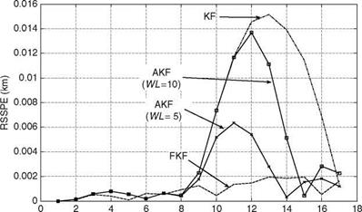
Scan number FIGURE 9.15 RSSPE for KF, FKF, and AKF for tracking of a maneuvering target (Example 9.3). |
P+ = P— — K(k)HP — (9.102)
1 k
A(k) = — ]T e(j)e(j)T; k > WL (9.103)
WL j=k-WL+1
Here, # stands for pseudo-inverse, e is the innovation sequence vector, and WL (= 5 for the present case) is the window length. It is important to note that online value of Q can be made available to AKF only from WLth scan, which means that accuracy of Q will depend on its initial guess (for k = 1to WLth — 1 scans) chosen by a filter designer. The AKF exhibited better tracking accuracy, especially during target maneuver, than KF but it had slightly degraded performance compared with FKF. For nonmaneuvering phases of target motion, AKF and KF perform almost similarly. During the maneuvering portion, it is found that the magnitude of online Q increases and so the Kalman gain; hence, automatically more weight is assigned to the measurement model, which aids in convergence of the estimated states to true values at a much faster rate than that seen for KF only. A sensitivity study of AKF with respect to different values of WL (5 and 10) was carried out and its performance in terms of RSSPE is compared with KF and FKF (Figure 9.15). It is observed that RSSPE of AKF during the maneuvering phase is high for WL = 10 as compared to WL = 5. This could be due to nonavailability of online Q and with an assumption that its initial guess is not sufficient at a time when actual maneuver starts, i. e., at k = 8.
It is essential to obtain accurate estimation of target states (position, velocity, and acceleration) from the noisy measurements originating from single or multiple sensors. KF is a suitable algorithm for such applications. In the case of multiple sources, either single KF can be used by fusing the measurements at data level or one can use state vector fusion. The accuracy of estimated/fused states depends on (1) how precisely the target and measurement models are known and (2) tuning parameters such as process noise covariance matrix “Q” and measurement noise covariance matrix ‘‘R,’’ which basically decide the bandwidth of the filter. In many situations, either mathematical models are not known accurately or are difficult to model. In practice, modeling errors are partially compensated by tuning Q, using trial
|
TABLE 9.14 Estimates by Adaptive Neuro-Fuzzy Inference System
|
and error or some heuristic approach. A fuzzy Kalman filter (FKF) is found suitable in such cases and it is investigated here. The performances of KF and FKF are compared with adaptive Kalman filter (AKF) in which the process noise covariance Q is computed online using the sliding window method.
FL is a multivalue logic (Chapter 2) used to model any event or condition that is not precisely defined or is unknown. In the FL-based system we use (1) membership function (fuzzification)—it converts the I/O crisp values to corresponding membership grades indicating its belongingness to respective fuzzy set; (2) rule base consisting of IF-THEN rules; (3) fuzzy implications used to map the fuzzified input to an appropriate fuzzified output; (4) aggregation used to combine the output fuzzy sets (single output fuzzy set for every rule fired) to single fuzzy set, and (5) defuzzification to convert the aggregated output fuzzy set from its fuzzified values to equivalent crisp values (Figure 2.20). In a KF, since the innovation sequence is the difference between sensor measurement and predicted value (based on the filter’s internal model), this mismatch can be used to perform the required adaptation using fuzzy logic rules. The advantages derived from the use of the fuzzy technique are the simplicity of the approach and the possibility of accommodating the heuristic knowledge about the phenomenon. This aspect is accommodated in Equation 9.44 as given by
X(k + 1/k + 1) = X(k + 1 /k) + KC(k + 1) (9.87)
Here, C(k + 1) is the fuzzy correlation variable (FCV) [36] and is a nonlinear function of the innovations vector e. It is assumed that target motion in each axis is independent. FCV consists of two inputs (i. e., ex and Єх) and single output cx(k + 1), where Єх is computed by
Here, T is the sampling time interval in seconds. In any FIS, fuzzy implication provides mapping between input and output fuzzy sets. Basically, a fuzzy IF-THEN rule is interpreted as a fuzzy implication. The antecedent membership functions would define the fuzzy values for inputs ex and ex. The labels used in linguistic variables to define membership functions are LN (large negative), MN (medium negative), SN (small negative), ZE (zero error), SP (small positive), MP (medium positive), and LP (large positive). The rules for the inference in FIS are created based on past experiences and intuitions. For example, one such rule is
If ex is LP and ex is LP then cx is LP (9.89)
This rule is created based on the fact that having ex and ex with large positive values indicates an increase in innovation sequence at a faster rate. The future value of ex (and therefore ex) can be reduced by increasing the present value of cx (a function of« Z — HX) with a large magnitude. Table 9.15 summarizes the 49 rules [36] used to implement FCV. Output cx at any instant of time can be computed using the inputs
 |
ex and ex, input membership functions, rules mentioned in Table 9.15, fuzzy inference engine, aggregator, and defuzzification.
The properties of FIS used in the present work are as follows: (1) its type is Mamdani; (2) AND operator is Min; (3) OR operator is Max; (4) implication used is Min; (5) Aggregation used is Max; and (6) the defuzzification used is Centroid (Figure 2.20).
Example 9.3: Target Tracking
The relevant MATLAB programs are “ExampSolSW/Example 9.3FKTT49Rules, 9.3FKTT4Rules, 9.3AKF.’’ The target data in x, y-direction are generated using the constant acceleration model with process noise increment [37]. With sampling interval T — 0.1 s, a total of N — 100 scans are generated. The data simulation proceeds with the following assumed parameter values and equations: (1) initial states of target x, x, x are 0 m, 100 m/s, and 0 m/s2, respectively, and initial states of y, y, у are 0 m,
— 100 m/s, and —10 m/s2, respectively; and (2) process noise variance Q — 0.0001. The target state equation is X(k + 1) — FX(k) + Gw(k) where, k is the scan number and w is the white Gaussian process noise with zero mean and covariance Q. The measurement equation is Zm(k) — HX(k) + v(k) with H — [1 0 0] and x and v are the measurement noise with zero mean and covariance R — S(s — 10 m). The system matrices are given as
 (9.90)
![]()
 |
|
|
||
|
|
|||
|
||||
|
||||
![]()
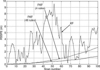
The initial conditions, F, G, H, Q, and R for both the filters are kept the same. The initial state vector X(0/0) is kept close to true initial states. The results for both the filters are compared in terms of true and estimated states and state errors with bounds at every scan number. Every effort was made to tune the KF properly. The same FCV is used for x, y-directions. The performances of both schemes are also compared in terms of RSSPE (root sum square position error) — J(x(k/k) — x(k/k))2 + (y(k/k) — y(k/k))2. Figure 9.13 compares the RSSPE computed using true and estimated states for both the filters. Although the performance of the KF is satisfactory and acceptable, the FKF performs better than the KF. For the same target data (i. e., x – and y-axes), the performance of KF with FKF is compared for two cases: (1) when all the 49 rules are taken into consideration and (2) when only 4 rules are used (Table 9.16).
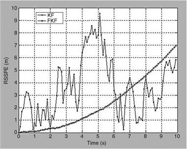 |
Figure 9.14 compares the RSSPE of FKF for these two cases. It is clear that the filter with 49 rules shows better performance than the filter with 4 rules, although the performance with 4 rules is quite acceptable. This indicates that to have a good FKF just a small number of rules is sufficient to obtain continuous and smooth I/O mapping. Too many rules are often unnecessary.
In recent times, approaches for parameter and state estimation using ANNs and fuzzy logic have improved. Here, some approaches are briefly discussed and a few results are given.
9.9.1 ANFIS for Parameter Estimation
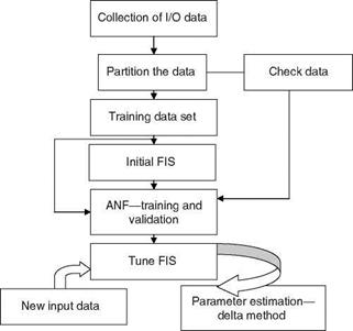
An ANFIS (the adaptive neuro-fuzzy inference system of MATLAB; MATLAB is a registered trademark of MathWorks, Inc.) for parameter estimation uses the rule – based procedure to represent the system behavior in the absence of a precise model of the system and uses the I/O data to determine the membership function’s parameters (constants). It consists of the fuzzy inference system (FIS) whose membership function’s parameters are tuned using either a back propagation algorithm or in combination with the LS method. These parameters will change through the learning process. The computation of these parameters is facilitated by a gradient vector, which provides a measure of how well the FIS models the I/O data for a given set of parameters. Once the gradient vector is obtained, any optimization routine can be applied to adjust the parameters to reduce the error measure defined by the sum of the squared difference of the actual and desired outputs. The membership function is adaptively tuned/determined using ANN and the I/O data of the given system. The FIS is shown in Figure 2.19. The process of system parameter estimation using ANFIS is depicted in Figure 9.11. The steps
|
|
|
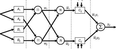
involved in the process are depicted in Figure 9.12. Consider a fuzzy system with the rule base: (1) If щ is Aj and u2 is Bb then yj = c11u1 + c12u2 + c10; if mj is A2 and u2 is B2, then y2 = c21uj + c22u2 + c20. Here, ub u2 are crisp/non-fuzzy inputs, and y is the desired output. Let the membership functions of fuzzy sets Ai, Bi, i = 1,2 be mA, mB. ‘ pi’’ is the product operator to combine the AND process of sets A and B, and N is the normalization. Cs are the output membership function parameters. The steps are given as (1) each neuron ‘‘i’’ in layer 1 is adaptive with a parametric activation function. Its output is the grade of membership function to which the given input satisfies the membership function, i. e., mA, mB. A generalized membership function m(u) = 1+|U-cj2b is used and the parameters (a, b, c) are premise
parameters; (2) every node in layer 2 is a fixed node, whose output (wi) is the product П of all incoming signals: w1 = mA (u1)mB (u2), i = 1,2; (3) output of layer 3 for each node is the ratio of the ith rule’s firing strength relative to the sum of all rules’ firing strengths: w, = www ; (4) every node in layer4 is an adaptive node with a node output: Wj-yj = w!(c! lu1 + ci2u2 + ci0), i = 1, 2. Here, c is the consequent parameters; and finally (5) every node in layer 5 is a fixed node, which sums all incoming signals yp = w1y1 + w2y2, where yp is the predicted output. When the parameters of the premise are fixed, the overall output is a linear combination of the consequent parameters. The output (linear in the consequent parameters) can be written as
yp = w 1y1 + W 2 y2 = w 1(c11U1 + c12U2 + c10) + W2(c21U1 + c22U2 + c2o)
= (w 1U1)c11 + (w1U2)c12 + w 1c10 + (w 2 U1)c21 + (w 2U2 )c22 + w 2c20
by the LS method. In a backward pass, the error signals propagate backward and the premise parameters are updated by a gradient descent method. The steps involved are (1) Generation of initial FIS by using INITFIS = genfis1(TRNDATA). ‘‘TRNDATA’’ is a matrix with N + 1 columns, where the first N columns contain data for each FIS, and the last column contains the output data. INITFIS is a single output FIS. (2) Training of FIS: [FIS, ERROR, STEPSIZE, CHKFIS, CHKERROR] = anfis(TRNDATA, INITFIS, TRNOPT, DISPOPT, CHKDATA). Here, vector TRNOPT represents training options, vector DISPOPT represents display options during training, CHKDATA prevents overfitting of the training data set, and CHKFIS is the final tuned FIS.
Example 9.2
Generate simulated data using the equation y = a + bxi + cx2, with a = 1, b = 2, and c = 1. Estimate the parameters a, b, c using ANFIS and the delta method.
Solution
The simulated data are generated and partitioned as training and check data sets. Then the training data are used to obtain tuned FIS, which is validated with the help of the check data set. The tuned FIS is, in turn, used to predict the system output for new input data of the same class and parameters estimated using the delta method. The MATLAB routines are given in ‘‘ExampSolSW/Example 9.2ANFISPEstm.’’ The results are shown in Table 9.14.
The idea is to estimate the parameters of a dynamic system
![]() 5c = Ax + Bu; x(0) = x0
5c = Ax + Bu; x(0) = x0
 |
Error
![]()
|
|
|
|
|
|
|
|
|
|
|
|
j=1
![]() + hi, j=i
+ hi, j=i
and since bi = f (Xi), and Xi = (f-1)’b,• dPi
we have, (f 1)’/3,• = —; hence
Comparing expressions from Equations 9.76 and 9.77 to Equation 9.80, the expressions for the weight matrix W and the bias vector b are obtained as
![Подпись: X21 X2X1 0 0 EUX1 0 EX1X2 X22 0 0 uX2 0 0 0 X21 X2X1 0 uX1 0 0 X1 X2 P X2 0 EUX2 X1 u EX2U 0 0 Eu2 0 0 0 X1 u EX2U 0 u2 EX 1x1 X]X 1X2 EX2X1 X]X2X2 EX 1U X]X 2И](/img/3131/image512_0.gif) (9.83)
(9.83)
(9.84)
The algorithm for parameter estimation of a dynamic system is given as follows: (1) as the measurements of X, X, and u are available for a certain time interval T, compute W matrix and bias vector b; (2) choose initial values of b randomly; and (3) solve the following differential equation.
Since bi = f (X;) and the sigmoid nonlinearities are known, by differentiating and simplifying, we get
Integration of Equation 9.85 would yield the solution to the parameter-estimation problem posed in equation error/RNN structure. Proper tuning of A and p is
essential. Often l is chosen as a small number, i. e., less than 1.0. The value of p is chosen such that when xt (of RNN) approaches ±1, f approaches ± p.
 |
9.8.1 FFNN Scheme
 |
We have seen that an FFNN can be used for nonlinear mapping of the input/output data. This suggests that it should be possible to use it for system identification/para – meter estimation. The FFNN works with a black-box model structure, which cannot be physically interpreted and hence the parameters, i. e., the network weights, have no interpretation in terms of the parameters of the actual system. The parameter estimation using FFNN is done in two steps: (1) the FFNN is presented with the measured data and trained to reproduce the clean/predicted responses, which are
Time (s)
FIGURE 9.9 Dynamic validation of global model of Cma from spline using 6DOF simulation. (From Shaik, I. and Singh, J., Aerodynamic Global Modeling Using Multivariate Orthogonal Functions and Splines, Accepted for presentation at the 20th National Convention of Aerospace Engineers, NCASE, Trivandrum, October 29-30, 2006. With permission.)
compared with the actual system’s responses in the sense of minimization of the output error as depicted in Figure 9.10 and (2) subsequently the predicted responses are perturbed in turn for each parameter that is to be estimated. This obtains a changed predicted response. Next, it is assumed that z = fix and the FFNN is trained to produce a clean z. Then the trained FFNN is used to produce z + Az and z — Az by changing x to x + Ax and x — Dx, and the parameter b is obtained as b = f+—x~. This is called the delta method. The estimates are obtained by averaging these respective parameter time histories, by removing some initial and some final points. The training algorithm for the FFNN is provided in Section 2.4.2.