Category FLIGHT MECHANICS MODELING and ANALYSIS

characteristics for large AOA range. Also, at certain flight conditions, it may not be possible to trim the aircraft and obtain the point models from the flight test data. Thus, global models obtained from the wind tunnel and flight data can constitute a total aerodynamic database, which would be a good source for validation of flight control performance, flight envelope expansion, and wind-tunnel aero database [31,32]. This aero database can be updated if required based on the results from flight test data analysis. A global model with a gradient and a large range of validity can replace many local models in the flight envelope. In addition, the partial derivatives of the global analytical model would provide point models (at trim conditions) that can be used in control system design. Multivariate orthogonal functions are very useful for global modeling of aerodynamic coefficients [31]. A minimum predicted squared error (PSE) criterion [1] can be used to determine the orthogonal functions to be included in the global model. The other criteria used are the sum of the conventional mean squared error (MSE) and an over-fit penalty (OFP) [33]. Each orthogonal function included in the global model can be decomposed into an ordinary polyno­mial in independent variables. Thus, the global model can assume the form of a truncated power series expansion, providing an insight into the physical relationship between the aerodynamic coefficients and independent variables. The orthogonal functions approach also allows for an easy upgrading of the model with the newly acquired flight data. Alternatively, the spline functions can be used to fit the flight – determined derivatives, padded with linear model derivative values obtained from wind-tunnel data, to determine global models of force and moment coefficients as functions of trim AOA and Mach number [34]. A spline is a smooth piecewise polynomial of degree m, with the function values and derivatives agreeing at the points where the piecewise polynomials join. These points are called ‘‘knots,’’ defined by the value of their projection on to the plane or axis of independent variables.

For the polynomial splines of degree m, a single variable function f(a) can be approximated in the interval a 2 [a0, amax] as

(9.70)

with

(a – a,)™ = (a – a,)m if (a > a,)

= 0 if (a < a,)

ab a2,ak are knots obeying the condition a0 < a1 < a2 < • •• < ak < amax and the coefficients Ch and D, are constants. A function of two variables f (a, b) can be approximated in the range, a Є [a0, amax] and b Є [bo, bmax], using polynomial splines in two variables. First-order splines are generally adequate for modeling the nondimensional derivatives of an aircraft. It is assumed that the spline polynomial of an aerodynamic derivative C, which is a function of a and Mach number, can be expressed as shown below:

k I

C(a, M) = Я00 + «0ia + ящМ + a\aM + E bi(a – a,)1 + Ec<M – M)1

i=1 j=1

k l

+ X) Edj(a – ai)1(M – Mj)1 (9.71)

i=1 j=1

Here, the constants a00, …a11, b,, c,-, and dj are to be determined. A higher order may be used if the degree of nonlinearity in the data is believed to be high. The LS regression matrix, computed using the values of the nondimensional derivative and the independent variables a and M, is orthogonalized using the Gram-Schimdt procedure. The minimum PSE metric is used to determine the model structure and the global model parameters are estimated using the LS regression method.

The global models of the nondimensional derivatives of a high-performance aircraft were identified using the splines technique and validated over an AOA range of 0°-22° and Mach range of 0.2-0.9 [33]. The GM of Cma from splines comprises 25 terms with the knots placed at every 1° a from 0° to 22°, and the Mach knots were placed at intervals of 0.1 between 0.2 and 0.9 Mach. According to Equation 9.70, as a increases, each spline function (a – ai) contributes less than the previous function, allowing for different values of derivatives to be computed for different values of a. The static validation of GMs is done by comparing them with several point values. The results of model fitting with splines are shown in Figures 9.7 through 9.9. GMs were validated dynamically using data from the 6DOF nonlinear simulation.

The usual procedure for aircraft parameter estimation is to perturb it slightly from its trim position by deflecting one or more of its control surfaces and gathering flight data from such small amplitude maneuvers. However, in practice it may not be possible to trim the aircraft at certain test points in the flight envelope. Under such conditions, large amplitude maneuvers (LAMs) are more useful in determining the aerodynamic derivatives. The approach is not valid in the region where stability and control derivatives vary rapidly. The results of the LAM are generated for the fighter aircraft FA2 for the conditions: (1) simulated longitudinal LAM data at two flight conditions and analyzed using the SMLR (stepwise multiple regression method [1]) without partitioning—here the entire data set is handled as a single LAM; (2) the data as in (1) but analyzed using the model error method (MEM [1]); and (3) the real flight data (*) analyzed using the previous two approaches [28]. The results are shown in Table 9.13.

The other method consists of partitioning the LAM that covers a large AOA range into several bins, each of which spans a smaller range of AOA [29]. These data would not be contiguous and therefore the regression method is employed to

TABLE 9.12 Fit Errors for Lift and Drag Coefficients—Parameter Estimation RC Maneuver Set 1 Set2 Set3 Set 4 Estimation Mach No. = 0.6 Mach No. = 0.7 Mach No. = 0.8 Mach No. = 1.0 Method Q CD Q Co Q Co Q Co EUDF-NMBA 0.0216 0.1586 0.0201 0.1112 0.0190 0.1036 0.0442 0.4275 EUDF-MBA 0.2597 0.9108 0.3940 0.6660 0.4939 1.0506 0.5439 0.3659 SOEM 0.2198 0.7540 0.3747 0.5979 0.4746 1.0009 0.4973 0.2996 WUT Maneuver Set 1 Set 2 Set 3 Set 4 Mach No. = 0.6 Mach No. = 0.7 Mach No. = 0.8 Mach No. = 1.0 EUDF-NMBA 0.0411 0.5960 0.0543 0.4930 0.0624 0.4588 0.0423 0.2261 EUDF-MBA 0.6193 0.9564 0.4524 1.1780 0.3922 0.8220 0.3995 0.7903 SOEM 0.3871 0.8862 0.4811 1.2402 0.5078 0.8579 0.2487 0.4741 Note: Altitude equal to 8 km.

TABLE 9.12 Fit Errors for Lift and Drag Coefficients—Parameter Estimation RC Maneuver Set 1 Set2 Set3 Set 4 Estimation Mach No. = 0.6 Mach No. = 0.7 Mach No. = 0.8 Mach No. = 1.0 Method Q CD Q Co Q Co Q Co EUDF-NMBA 0.0216 0.1586 0.0201 0.1112 0.0190 0.1036 0.0442 0.4275 EUDF-MBA 0.2597 0.9108 0.3940 0.6660 0.4939 1.0506 0.5439 0.3659 SOEM 0.2198 0.7540 0.3747 0.5979 0.4746 1.0009 0.4973 0.2996 WUT Maneuver Set 1 Set 2 Set 3 Set 4 Mach No. = 0.6 Mach No. = 0.7 Mach No. = 0.8 Mach No. = 1.0 EUDF-NMBA 0.0411 0.5960 0.0543 0.4930 0.0624 0.4588 0.0423 0.2261 EUDF-MBA 0.6193 0.9564 0.4524 1.1780 0.3922 0.8220 0.3995 0.7903 SOEM 0.3871 0.8862 0.4811 1.2402 0.5078 0.8579 0.2487 0.4741 Note: Altitude equal to 8 km.

estimate derivatives. This approach was also used for the analysis of the data mentioned earlier, and the detailed results can be found in Ref. [28].

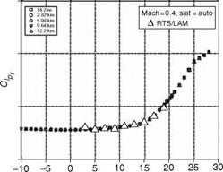
For LD data generation from LAMs (in an RTS), the modes were excited in roll and yaw axes by giving aileron and rudder inputs superimposed on a steadily increasing AOA due to slow but steady increase in elevator deflection, thereby generating LAM data. Normal practice is to estimate linear derivative models but, if necessary, the SMLR approach can be used to determine the model structure with higher-order terms for better representation of aircraft dynamics. A pilot flew an RTS (Chapter 6) and persistently excited the roll and yaw motions at increasing AOA in pullup. The data were generated for Mach numbers 0.4 and 0.6 with AOA variation between 2° and 20° [30]. Significant variation in yaw during lateral stick inputs, possibly caused by aileron-rudder interconnect, was seen in the time – history plots. Regression and data partitioning techniques were used for estimation of the LD derivatives. For each Mach, the data were partitioned into bins, where each bin corresponds to a mean value of AOA: at Mach 0.4, the total variation in AOA is from 2° to 20°. The data from 2° to 4° are put into one group; the data from 4° to 6° are put into another group, and so on until all the data are accounted for. The data in a group would have resulted from different portions of a single maneuver or from certain portions of several other maneuvers. These data in each group were analyzed using regression. Each bin should have sufficient number of data points for successful estimation of derivatives and should have sufficient variations in the aircraft motion variables so that accurate estimation of derivatives is possible. Several criteria, e. g., the number of data points in each bin, the CRBs of the estimated derivatives, and the percentage fit error, were evaluated to check the quality of the estimates. The derivatives C„b, C/, C„v and C/ were estimated and cross-plotted with the reference derivatives. The results were very encouraging. One compound derivative (for the flight condition Mach number = 0.6 and with auto slat) C = C^ + Q tan a is shown Figure 9.6 [30]. This RTS exercise established that the approach if followed would work for the data gathered from real flight tests. Using this approach it is possible to determine the aerodynamic derivatives at flight conditions that cannot be covered during 1g trim flight.

(1) Suboptimal smoothed states of an aircraft are obtained using the EKF-smoother [1,14]. Scale factors and bias errors in the sensors are estimated using the data compatibility checking procedure. (2) The aerodynamic lift and drag coefficients are computed using the corrected measurements (from step 1) of the forward and normal accelerations using the following relations:

(9.68)

The lift and drag coefficients are computed from Cx and Cz using

CL = —Cz cos a + CX sin a CD = — CX cos a — Cz sin a

CD versus CL is plotted to obtain the drag polar. The first step could be accomplished using the state and measurement models for kinematic consistency. Typical results of this case study are shown in Table 9.12.

The indicated maneuvers (Chapter 7) were performed on a supersonic fighter aircraft at several flight conditions. We can easily see from Table 9.12 that the non­model-based approach (EUDF-NMBA) gives better fit (lesser percentage fit errors) to the data and hence accurate determination of the drag polars from flight data. An NMBA could be preferred over a model-based approach as it requires less computation time and still gives accurate results for drag polars from flight data and is a potential method for real-time online determination of drag polars.

In the model-based method, an explicit aerodynamic model for lift and drag coeffi­cients is formulated as shown below:

State model:

cfS F

V =———- CD H——- e cos (a + sT) + g sin (a — в)

mm

a = —_Й^_ cl – — sin (a + sT) + q + — cos (a — в) (9-65)

mV mV 4 V

в = q

Here, CL and CD are modeled as

V qc

CL = CLo + CLy— H CLaa + CLq~—— H CLSe de

u-o 2Uo

CD = CDo + CDV – H CDaa + CDa2 a2 + CDq —- H CDSede

Uo 2Uo

Observation model:

VV

v m v

The aerodynamic derivatives in the above equations could be estimated using OEM for stable aircraft (stabilized OEM for unstable aircraft) or using extended unit upper triangular-diagonal (UD) filter. In the extended KF, the aerodynamic derivatives in Equation 9.66 would form part of the augmented state model. The estimated CL and CD are then used to generate the drag polars [16,25-27].

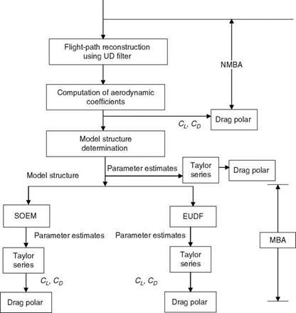
The estimation of drag polars (drag coefficient vs. lift coefficient) is an important activity in any aircraft development/flight-test program. Drag polar data are required to assess the actual performance capability of the aircraft from flight test data. Dynamic flight test maneuvers of various types [25,26] can be performed on an aircraft and the data analyzed using OEM for a stable aircraft and SOEMs for unstable/augmented aircraft. Dynamic maneuvers such as RC, SD, and WUT are most suitable for drag polar determination. Model-based and non-model-based approaches are suitable for determination of drag polars and these are linked in Figure 9.5 [27]. The estimation before the modeling method can be used to

determine the structure of the aerodynamic model to be used in the model-based approach.

An attempt was made to analyze the SP maneuver data generated from an iron bird (IB) for a fighter aircraft with the following flight condition: Mach number = 0.41, H = 3 km, undercarriage down, and alpha trim = 7.69°. An SP maneuver was excited with a pitch stick command input doublet. The pulse width was 2.8 s, and the sampling rate was 40 samples/s, and 320 data points were available for parameter estimation. The estimation results are compared with those from flight simulation (FS) and nondimensional linear (NLM) model parameters in Table 9.11. The results seem satisfactory.

It is seen that for this flight condition the aircraft is almost statically-neutrally stable or unstable. The pitch damping is also poor. It must be emphasized here that the open loop dynamics of this aircraft are unstable, and it operates in a closed loop with a control system.

Dynamic wind-tunnel (DWT, NAL) experiments on a scaled (-down) model of a delta-wing aircraft were conducted using a single degree of freedom in pitch, yaw, and roll. The DWT facility is a 1.2 m x 1.2 m low-speed (20 to 60 m/s) tunnel of open jet – induced draft type. The FRP aircraft model was supported at the back on a low friction

bearing assembly for the roll motion experiments. DC motors drove the elevons of the aircraft model. In the DWT experiment the aircraft model is free to move about a gimbal with translational and rotary degrees of freedom. The experiments are of semi­free flying type as against the conventional/static wind-tunnel experiments. Miniature (incidence), rate, and acceleration sensors were mounted inside the hollow model of the aircraft to pick up the dynamic responses to the given inputs. Control surface movements were measured using precision potentiometers. Angular accelerations were sensed using a set of strain gauge type accelerometers. The test inputs were applied to servo-controlled (control) surfaces to excite the modes of the aircraft model. Aerodynamic derivatives were estimated from the motion responses of the model by using OEM and the results were compared with other wind-tunnel test methods [24]. The estimated derivatives are given in Table 9.10.

In this study, the OEM is used for estimation of the aerodynamic derivatives of AGARD standard ballistic model (SBM) from the data available in the open literature. For this SBM, the hybrid model with aerodynamic forces represented in the wind axis and the moments in the body axis coordinate systems was used [23]. The SBM is composed of a blunt nose cone with a cylindrical midsection followed by a 10° flare. This axis-symmetric, uninstrumented model is solid in construction. The free-light tests were performed at Mach number 2.0 in the NASA Ames pressurized ballistic range facility. The model, as it flew the down range, was photographed by 22 fully instrumented orthogonal shadowgraph stations. The trans­lational and angular motions were acquired in Earth-fixed orthogonal coordinates based on analysis of the film records. The NASA method was based on the LS/Gaussian LS differential approach. The V-a, b and the body axis models were used. The available data for V, x, y, z, U, w in a short flight duration were not uniformly sampled and hence a cubic spline interpolation was used to generate uniform data sets. The flow angle trajectories were generated using a = U + tan_1(dz/dx) and b = —■f + tan_1(dy/dx). Table 9.9 shows a comparison of some of the aerodynamic derivatives.

Due to the axis-symmetry property of the AGARD SBM, the static stability derivatives in longitudinal and lateral axes are the same except for the polarity.

Light canard research aircraft (LCRA) is an all-composite aircraft with canard and is based on the Rutan long-EZ design. It is a two-seater aircraft with pusher propeller and has a tricycle landing gear with retractable nose wheel. The wings have moderate sweeps and the canard has trailing edge flaps that function as the elevators. The LCRA has two rudders. The ailerons are situated in the wings. SP and DR maneuvers were carried out at altitude = 1.53 and 2.74 km and at three speeds 65, 85, and 105 knots at each altitude. Table 9.6 shows the comparison of the analytical (values that were almost constant) and the average values of FDDs of LCRA for longitudinal and LD axes. The scatter and the CRBs for most of the estimated derivatives were reasonably low [21]. Also, SP natural frequency and damping ratio were fairly constant over the AOA range and hence average values are given in Table 9.6. The asterisk (*) indicates that there is a slight trend of the damping-in-roll derivative (C) with AOA and signifies the reduction in the damping with increasing AOA, whereas the analytical value is constant. This shows that the flight data provides additional information and hence enhanced confidence in the dynamic characteristics of the vehicle. This exercise shows that for this light and small aircraft, the aerody­namics are fairly linear with respect to AOA. It also shows that though the FDDs are not far away from the analytical values, the pitch and directional static stability are reduced in flight. However, the dihedral static stability is increased.

9.4.5 Helicopter

The flight tests on a helicopter consisted of 14 sets of recorded data runs at the uniform sampling rate of 8 samples/s. The longitudinal modes were excited by

applying a doublet input command and a 3-2-1-1 like input for the longitudinal cyclic control, and lateral maneuver was excited. The longitudinal derivatives are shown in Table 9.7. Since the reference values were not available, no comparison could be made with the FDDs. Hence, the approach used was to analyze the individual data sets and also to use the corresponding data in a multiple maneuver analysis mode. The latter involves the concatenation of the time histories of the repeat runs (obtained at the same flight conditions) and use in the OEM such that average results are obtained. Since the results from both these approaches were almost identical, except for a few cases, and the estimates had low CRBs, the FDDs were believed to be of acceptable values. In most aircraft parameter-estimation applications, the forces and moments acting on the aircraft are approximated by terms in Taylor’s series expansion, resulting in a model that is linear in parameters. However, when the aerodynamic characteristics are rapidly changing, mathematical that have more num­ber of parameters and cross derivatives may be required. Table 9.8 gives the lateral FDDs of the helicopter estimated with and without cross derivatives. The improve­ment in the lateral velocity component and yaw rate response match is observed when cross-coupled derivatives Nu, Nw, and Nq are included in the yawing moment equation

during estimation. With cross-coupled derivatives included, estimated values of other yaw derivatives, particularly Nr, register a change resulting in improved match. The time-history match with flight data improved when the model included some cross­coupled derivatives [22]. This aspect is important for the flight data analysis of a helicopter. The search for obtaining adequate aerodynamic models that can satisfac­torily represent the helicopter characteristics can be further pursued using SMLR and the model error estimation (MEE) method.

The basic jet trainer is a two-seater low-wing monoplane aircraft. The flight tests were carried out by AFTPS (Air force Test Pilots School, Aircraft Systems and Testing Establishment) at 4570 and 6700 m altitudes on this aircraft. The sampling interval for data acquisition was 31.25 ms. The flight-determined values are Cm =—0.5, Cm = —15, and CLa = 4.9 (WT value is 4.5). The latter derivative was fairly constant as the lift curve fairly and monotonically increased up to AOA of 12°. In the range of AOA = 8°-12°, the SP frequency was 1.5 rad/s and at low AOA it was 3 rad/s, whereas the SP damping ratio was fairly constant at the average value of 0.45 [20]. Another jet trainer version has the following characteristics determined from the specific flight tests conducted (at M = 0.5, 0.6, 0.7, and H = 5000 m; CG = 27.5%

MAC): NP = 32.5% of MAC; SP frequency = 2.5 rad/s; SP damping ratio = 0.4; the phugoid frequency = 0.08, and the damping ratio = 0.11.