Category Management and Minimisation of Uncertainties and Errors in Numerical Aerodynamics

Implementation of the Separation Sensor

As already mentioned the development of the boundary layer with different turbu­lence models leads to different gradients in the friction coefficients. This implies, depending on the position and choice of model, a premature or delayed separation. A constant dependence between model and separation is not identifiable. The user only gets a feedback about an existing separation effect and the critical areas are marked as a surface value in the output files. To detect the appearance of separation

Implementation of the Separation Sensor

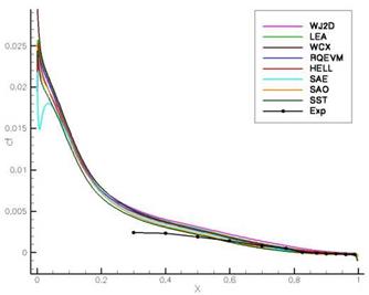
Fig. 12 ONERA-A — friction coefficient Cf in comparision with the eight different turbu­lence models and the experiment

the sensor scans the surface for characteristic points (first order) of separation or reat­tachment. For this every surface triangle is tested. Every triangle element which con­tains two zero-crossings along the edges in the wall-tangential velocities includes a critical point. In the code the velocity at the wall is represented by the components of Cf. These marked elements include hyperbolic points (the beginning or end of a separation line) or rotation points (a vortex separation). To exclude stagnation areas a minimal pressure coefficient of cp < 0.5 is assumed.

Separation

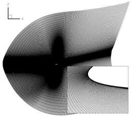
The quality of the different turbulence models to predict the correct position of a separation is very variable. This has a great influence on the correct prediction of the drag and lift coefficients. For the investigation the 2D test-case Onera-A at13.3 angle of attack was chosen. The test-case has a separation at 89.5% chord-length on the suction side with Re = 2.1e6 and Ma = 0.15. The grid consists of 530,000 grid points (fig. 10) and was already tested on grid convergence in the ECARP-project. The order of convergence of the turbulence models differs slightly, but the results should also be comparable.

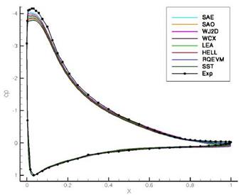
The variation of the turbulence models leads to visible variations in the separ­ation position and also to different levels in Cp and Cf (fig. 11 & 12). Compared to the experiment the deviations are 8.9% in the lift and up to 73.62% in the drag coefficient (SST). This strong deviation in the drag coefficient is in part due to the fully-turbulent computations applied: A user-specified transition location is known to ignore results for this test case. The range of variation in the forces reaches

Separation

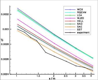
Fig. 9 Flat plate — friction coefficient cf with variation of the turbulence model in compar – ision to the experiment


Separation

Fig. 10 Grid of the ONERA-A test-case with 530,000 grid points


+/ — 3.56% in the lift, +/ — 3.43% in the drag coefficient and +/ — 7.69% in the position of the separation around the average of the numerical results.


Separation

Fig. 11 ONERA-A — pressure coefficient Cp in comparision with the eight different turbu­lence models and the experiment

Table 1 ONERA-A – lift and drag coefficient, position of pressure induced separation com­pared to experimental results

CL

diff. in % cd

diff. in % separation

x/c

diff. in %

Experiment

1.5620

0.0208

0.8945

HELL

1.4480

-7.30

0.0356

70.96

0.8906

-0.44

LEA

1.4659

-6.15

0.0347

66.92

0.9228

3.16

RQEVM

1.4234

-8.87

0.0351

68.90

0.8883

-0.70

SAE

1.5275

-2.21

0.0337

62.12

0.8312

-7.08

SAO

1.5119

-3.21

0.0350

68.38

0.8078

-9.69

SST

1.4225

-8.93

0.0361

73.62

0.8268

-7.57

WCX

1.4857

-4.89

0.0352

69.08

0.8976

0.35

WJ2D

1.5081

-3.45

0.0342

64.59

0.9423

5.35

Implementation of the Boundary Layer Sensor

For the implementation of this sensor again the boundary layer has to be scanned to identify their thickness and the number of wall normal grid points. As the investiga­tions show the choice of the turbulence model itself is an uncertainty. Depending on the model the boundary layer thickness or the friction is differing to each other. The greatest problem is the difference in the gradients of the various values especially the friction coefficient. The reason for this is the calibration of the models and their

Implementation of the Boundary Layer Sensor

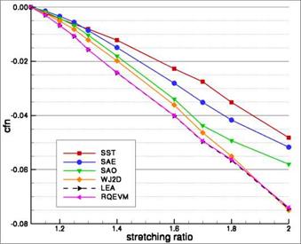
Fig. 8 Flat plate — influence of the grid expansion ratio on the prediction of the friction coefficient Cf, normalized with Cf of the reference grid with Menter SST, SAE, SAO, Wallin & Johansson EARSM, RQEVM and LEA model

different development of the boundary layer. Hence it is impossible to give a correct prediction for a local error. Despite that the sensor gives feedback to the user about the boundary layer thickness and the applied grid resolution.

Boundary Layer

For the investigation of the model dependencies on boundary layer development again the flat plate test-case was applied. The grid is identical as the reference grid for the error analysis.

The variation of the turbulence model leads to visible differences in the friction coefficients and boundary layer thickness (fig. 9). Here the results and the experi­mental data were compared at given positions x. In comparison to the experiment the simulations show differences in the fully developed boundary layer at x = 4.124m of up to 26.4% in the boundary layer thickness delta (WCX) and 6.7% in the friction coefficients Cf. The error range of the different models is +/ — 12.71% in 8 and +/ — 3.58% based on an average value over all models.

Development ofthe Uncertainty Sensors

As already mentioned, the uncertainties considered are mostly model-related and can be the result of the specification or weaknesses of the model itself. Reasons for uncertainties could be a lack of information of the physical background of the investigated flow problem.

Development ofthe Uncertainty Sensors

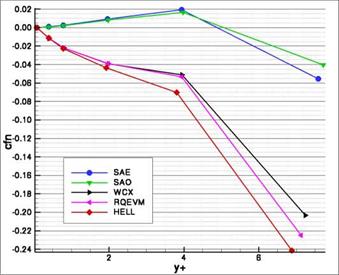
Fig. 7 Flat plate — influence of the wall distance y+ on the prediction of the friction coef­ficient Cf, normalized with Cf of the reference grid with SAE, SAO, Hellsten EARSM, RQEVM and Wilcox k-w model

Maximum Grid Expansion Ratio in the Boundary Layer Resolution

For the investigation of the near wall grid expansion the reference grid is again used as a basis. The expansion ratio was varied between r = 1.1 up to r = 2.0. Again all eight turbulence models were applied.

In the results with small variations the influence of the expansion ratio could be seen clearly. The behavior of the error prediction with different turbulence models is similar (Fig. 8). With a bigger ratio upto r = 2.0, the differences to the reference solution lead to 8% in the friction coefficients Cf in some cases. Greater values of the expansion ratio weren’t investigated. To ensure that the error prediction doesn’t depend on the local streamwise position within the boundary layer, the normalized

Maximum Grid Expansion Ratio in the Boundary Layer Resolution

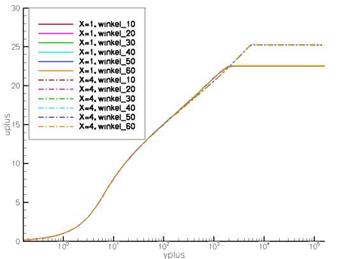
Fig. 3 Flat plate — WCX model — graph of u+ /y+ with variations of grid inclination in the boundary layer at x = 1.021 and x = 4. 124

Maximum Grid Expansion Ratio in the Boundary Layer Resolution

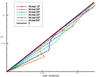
Fig. 4 Computation of the wall distance in TAU with variations of the grid inclination in the boundary layer in comparision to the correct wall distance z

Maximum Grid Expansion Ratio in the Boundary Layer Resolution

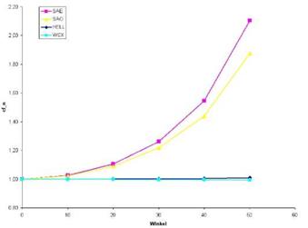
Fig. 5 Flat plate — influence of the grid inclination on the prediction of the friction coef­ficient Cf, normalized with Cf of the reference grid with SAE, SAO, Hellsten EARSM and Wilcox k-m model

error factor of friction Cfn has been evaluated at several positions. The behaviors of Cfn over r as well as y+ were compared between these locations. As the compar­ison of the cfn progression reveals, the error predictions are nearly identical at all

Maximum Grid Expansion Ratio in the Boundary Layer Resolution

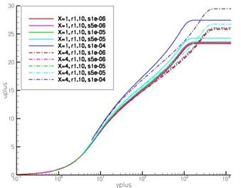
Fig. 6 Flat plate — Hellsten EARSM model — graph of u+ /y+ with variations of y+ at x = 1.021 and x = 4.124

positions. A minimal deviation occurs only at high levels of y+ and r. According to that Cfn can be assumed independent of the stream-wise location in boundary layer.

Implementation of the Expansion Sensor

For the implementation of the sensor for the expansion ratio again the boundary layer has to be scanned. The identified maximal ratio is assumed as constant at the related surface grid point. The behavior of the error was parameterized with a polynomial 3rd order for each turbulence model. This polynomial again represents the difference to the results with the reference grid in %. The difference is set to 100% if the expansion ratio leaves the investigated range of values.

Implementation of the y+ Sensor

For the implementation of the y+-sensor the behavior of the error was parameterized with a polynomial 3rd order for each turbulence model. The polynomial represents the difference to the results with the reference grid in %. Because of the low-Re boundary condition and the lack of error data for y+ > 7, the difference is set to 100% if y+ exceeds the viscous sub-layer.

Wall Distance y+

Again the reference grid was the basis for the investigations of the normalized wall distance y+. For this the wall nearest grid point was varied between y+ = 0.07 to y+= 7.

In the results (Fig. 6) a high sensitivity to the wall distance y+ is seen, with a widening of the boundary layer and modification of Tw, and hence uT. Depending on the model, at y+ « 1 these values achieve differences up to 2.5% compared to the reference computations. With further variations the differences exceed 25% quite fast. As the figure 7 shows, the behavior of the error in Cf is independent of the position in the boundary layer. y+ > 7 leads to divergence of the simulations or

зо

Wall Distance y+

yplus

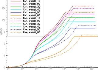
Fig. 2 Flat plate — SAE model — graph of u+ /y+ with variations of grid inclination in the boundary layer at x = 1.021 and x = 4.124

unexpected results. The results shown all apply the default low-Re wall treatment and the use of wall functions were not examined.

Implementation of the Inclinitation Sensor

For an automatic evaluation by the flow solver of the boundary layer thickness, the grid stretching ratio and the skewness near the wall, the boundary layer had to been scanned at every grid point on the surface. For this, the neighboring point furthest from the wall was detected, starting at each surface point and working in the wall normal direction. In this manner the entire boundary layer is traversed until the total pressure reaches 99.9% of the free stream total pressure [2]. The skewness of the grid is defined as the average deviation from the wall normal vector and the stretch­ing ratio as the maximum stretching ratio found inside the boundary layer. These quantities are saved at the respective surface points. From the results of the test computations for the isolated error mechanisms the magnitude of the expected er­ror was determined. The friction coefficient at the positions x1…x4 was computed

Implementation of the Inclinitation Sensor

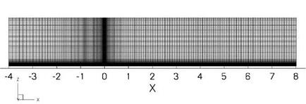
Fig. 1 Structured grid of the flat plate test-case with 52,000 grid points

and compared by normalization with the results of the reference grid. The error factor of Cf is therefore given by

and the percentage error as Cfn ■ 100%. This was carried out for all four stream – wise positions to verify independence of this variable. For the prediction of the errors in cf the skewness is assumed as constant. The error factor cfn was para­meterized with a 3rd order polynomial (p(x) = a0 + a]_x + a2x2 + a3x3 ) and the coefficients ai were identified for all investigated models.

Orthogonality in the Boundary Layer

To investigate the influence of the inclination of the grid in the boundary layer the reference grid (y0 = 1e – 6, y+ = 0.08, ratio = 1.1) were inclined to achieve angle variations of 0deg to 70deg in 10deg steps. Angles against the flow direction were tested only between – 10deg and -30deg. Here the results show the same influence as the angles in the flow direction. Hence the independence of the angle direction is assumed.

The variation of the inclination in the boundary layer shows with the one – equation models (SAO and SAE) a massive influence in the results (fig. 2 & 3). Compared with the results of the reference grid the friction coefficients differ by more than 100% at an inclination of 60deg (fig. 5). The same behavior is shown in the drag coefficient cD. This influence is however the result of inaccuracies arising from the computation of the wall-normal distance d (fig. 4), which is reflected most strongly in the results of the models with the strongest dependency on d. A lower er­ror occurs with the models SST and Hellsten EARSM and the error is negliable for the remaining models. With increasing inclination the calculated wall distance dif­fers from the correct values. This leads to the demonstrated errors with all turbulence models that depend on the wall distance. For this simple geometry, the analytically correct value of d could easily be determined. Replacing the computed d with the correct value gave results with negliable sensitvity to the grid inclination.