Category Management and Minimisation of Uncertainties and Errors in Numerical Aerodynamics

The Taguchi-Method

Subsequently the basic ideas of the Taguchi method are summarized. For more in­formation it is referred to [2] to [6].

The Taguchi Method is based on the DoE-Method (Design of Experiments). DoE is a statistical method for quality management, usually used for the optimization of production cycles by determining the influence of chosen parameters on the quality of the final product. The aim of the DoE to is reduce the number of experiments needed to evaluate the influences of the parameters to a minimum in comparison to a full parameter variation. Especially the method developed by Gen’ichi Taguchi (born 1924) using orthogonal arrays for the experiment setup needs only a minimum of numbers of experiments [2]. The number of experiments required for a full para­meter analysis rises exponential with the number of investigated parameters and the number of levels. If the influences of 4 parameters with 3 levels each should be investigated 34 = 81 experiments would be necessary. In the case of 13 parameters with 3 levels 2197 experiments should be done. The Taguchi method needs for these cases only 9 and 27 experiments respectively. This results in a much shorter simu­lation time and less required resources. Another advantage of the Taguchi-Method is the possibility to evaluate also the effects of interactions between the parameters.

In the present investigations the Taguchi method is applied to assess the impact of different parameter settings on the results of CFD simulations. These results can be the calculated lift or the different drag portions (viscous drag and pressure drag). It enables to investigate several numerical and geometrical parameters in a very short time with an acceptable number of CFD analyses.

A

В

C

D

1

1

1

1

1

R1

2

1

2

2

2

R2

3

1

3

3

3

R3

4

2

1

2

3

R4

5

2

2

3

1

R5

6

2

3

1

2

R6

7

3

1

3

2

R7

8

3

2

1

3

R8

9

3

3

2

1

R9

Fig. 1 L9-Taguchi-Matrix
Statistical Analysis of Parameter Variations Using the Taguchi Method

A. Wolf, D. Henes, S. Bogdanski, Th. Lutz, and E. Kramer

Abstract. This project is part of the MUNA-project. It deals with the investigations of uncertainties of a CFD-Simulation caused by variation of numerical parameters, inflow conditions and geometrical parameters. To evaluate the influence of different parameters on the results of an experiment or simulation usually a full parameter analysis must be performed. A full parameter analysis requires a high number of simulations, rising with the number of parameters, which are investigated. In this study the Taguchi method, which is based on DoE (Design of Experiments) meth­ods and well known for the optimization of production cycles, is applied. It reduces the number of required simulations dramatically and therefore also the costs. In this article the basics of the Taguchi Method are explained and a summary of the ANOVA-analysis, is given. The ANOVA analysis is used for the analysis of the results obtained by the Taguchi method. It delivers the relative influences of each investigated parameter and also the influence of interaction among different para­meters can be obtained. The effect of the parameter variations on the CFD result is shown for two – and three dimensional simulations. Numerical, geometrical and also inflow conditions are investigated.

1 Introduction

The aim of this project is to investigate the uncertainties in CFD-results if differ­ent numerical (i. e numerical diffusion) and geometrical (i. e. trailing edge thickness) parameters are varied. Most of the settings used for CFD simulations are based on experience and it is unknown how the result behaves if these parameters are

A. Wolf • D. Henes • S. Bogdanski • Th. Lutz • E. Kramer Institute of Aerodynamics and Gasdynamics, University of Stuttgart e-mail: wolf, lutz@iag. uni-stuttgart. de,

Pfaffenwaldring 21, 70569 Stuttgart

B. Eisfeld et al. (Eds.): Management & Minimisation of Uncert. & Errors, NNFM 122, pp. 247-264. DOI: 10.1007/978-3-642-36185-2_10 © Springer-Verlag Berlin Heidelberg 2013

changed. On the other hand there are also natural variations like fluctuating inflow conditions and production inaccuracies. Their effect is unknown as well. To eval­uate the influence of all these parameters, usually a full parameter analysis must be performed. As such an analysis requires several thousand simulations, the Tagu- chi method is introduced in this article, which requires a much lower number of simulations. The Taguchi method enables to investigate the relative influence of dif­ferent parameters on the CFD result by systematical variation of these parameters. It also enables to investigate the effect of the interactions between two parameters. It could be shown that in some cases the strongest influences on the CFD results stem from such interaction effects. In the first part of this article the Taguchi Method is explained and the results of the simulations are presented in the second part. The parameters are arranged in different groups depending whether they are numerical based, geometrical based or belong to inflow conditions. As test case the RAE2822 is chosen. The inflow conditions are taken from [1].

Summary

This work has presented a mesh deformation module for the parallel simulation environment FlowSimulator. The module is based on the radial basis function inter­polation approach.

Summary

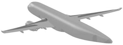
Fig. 14 Complex high-lift configuration for a CFD/CSM coupled simulation applying the new tool FSDeformation. Shown is the deformed and non-deformed geometry (see wing tip) due to a different aerodynamic load case.

The application fields of mesh deformation is manifold (unsteady simulations, shape optimization and aeroelasticity). In a next step, radial basis function inter­polation and the mesh deformation module and its algorithm have been introduced. The module combines the radial basis function interpolation approach with a group­weighting and deformation-blending feature. This allows to move different surface groups/bodies independently from each other. Furthermore, the deformation blend­ing provides an improved protection of boundary layer cells and allows the usage of unbounded radial basis functions and the extension of the radial basis function interpolation approach by a polynomial.

The group-weighting and deformation-blending uses the wall distance of the volume mesh nodes to the group boundaries. Hence a wall distance computation module has been implemented. It uses an advancing-front algorithm for the distance computation.

Additionally, the deformation module was extended with new deformation group features. These features allow to define deformation groups without creating base points and deformation vectors for this group. The features support far-field bound­aries, symmetry planes or the rigid attachment of a boundary group to another boundary group.

Because the computational cost of the interpolation algorithm depends on the number of interpolation base points, the module offers four different methods for the reduction of the input base points. The first method uses an octree data-structure to select equidistant base points. The remaining three methods use in the first step this method as well. But in the second step they either use weighted distances for a modified equidistant reduction function, or they correct the interpolation error locally by selecting base points individually. The two weighted distance reduction methods use the difference to the mean deformation of the neighboring nodes or the interpolation error of the base points not selected for the weight computation. All the different methods have been compared in terms of performance and inter­polation error. Here the locally operating error correction method has shown very good results in performance/interpolation error efficiency. But the method is limited to locally supported radial basis functions. Because the radial basis function Euc­lid’s Hat, which tends to infinity for an increasing input argument, has produced the lowest interpolation error, the interpolation error weighting method is the best advice.

The wall distance module and the deformation module have been parallelized with MPI. The theoretically perfect speedup of the interpolation method may only be affected by unbalanced node distributions over the parallel MPI processes.

The creation of the module FSDeformation by Airbus and its integration into the parallel FlowSimulator software environment has helped to reduce the uncertainties that occur in small geometry changes, which typically occur at aerodynamic shape design. Numerical shape optimization of components by using the improved grid deformation technique for unstructured grids has improved, reducing uncertainties related to mesh dependencies of the numerically obtained flow solutions.

Finally, applications for the deformation module in cooperation with the flow solver TAU and a structure module has been demonstrated. It has shown that the deformation module can play a key position in future computation chains using the simulation environment FlowSimulator with a perfect speedup for the mesh deform­ation method. Additionally, the example has illustrated that the coupling of different programs by using FlowSimulator can minimize intensive and time-consuming file input/output operations, due to the fact that both tools use the same main memory address space. The computational time and hence the cost of an optimization has been reduced considerably.

Application to Complex Configuration

It was found that FSDeformation in the parallel FlowSimulator environment could be applied successfully to very complex, industrially relevant problems. An example for a coupled CFD/CSM application for an complete aircraft in high-lift configura­tion with deflected flaps and slats is shown in Fig. 14.

Application to Complex Configuration

(a) Side view to check change of bend and twist. Lower wing: optimized, Upper wing: initial

Application to Complex Configuration
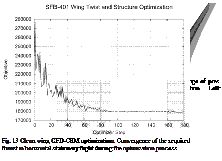
Fig. 12 Clean wing CFD-CSM optimization

Multi-disciplinary Wing Optimization-SFB-401-Wing

The task given was to optimize a wing with respect to aerodynamics, structures, and performance under considerations of static aeroelastic effects. The study involves the sizing of the wing box skins and spars to obtain minimum weight fulfilling static aero-elastic requirements (details in [7, p. 287]).

The considered MDO process chain for shape optimization of a wing including the static deformation is shown schematically in Fig. 1. The objective function is:

Obj = Wa/c x Cd/Cl, (44)

where Wa/c is the total weight of the aircraft, Cd is the overall aerodynamic drag coefficient, and Cl is the aerodynamic lift coefficient. The objective, thrust, is equi­valent to the total aerodynamic drag force in stationary horizontal flight, which should be minimized.

A CATIA V5 parametric model of the wing is controlled by the optimizer using an external CATIA-DesignTable, where all relevant shape parameters for the wing are listed. The shape of airfoils at four predefined wing sections (root, kink1, kink2, and tip section) can be changed parametrically to control the thickness, camber, and twist distribution of the wing. The wing planform is fixed.

Two structure design parameters control the relative thickness change of the wing front and rear spars in combination with the upper and lower sheet thicknesses of the

Multi-disciplinary Wing Optimization-SFB-401-Wing

(a) Step 1, no deformation (b) Step 10, aeroelastic equilibrium

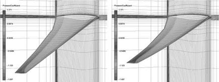
Fig. 11 Undeformed and deformed wing with pressure coefficient distribution and CFD mesh for the CFD/CSM coupled iterative process.

wing box. The stiffness and the weight of the wing are depending on these structure parameters.

Mesh deformation is a crucial component here. On the one hand, the change in geometry shape design through the parametric CAD model (CATIA V5) is treated by mesh deformation, on the other hand, the deformation of the wing structure de­pending on the aerodynamic forces (in addition to other forces such as fuel weight, engines, etc.) is also covered by applying mesh deformation. The CFD/CSM coup­ling is displayed in figure 11.

The individual components of the process chain were used in the parallel, in­memory FlowSimulator environment [1], so that a time-consuming and data intens­ive exchange of files was not required. Compared to the former methods, which used file exchange, significant time savings of around 50 percent have been ob­tained. This a major step forward in an industrial context together with the accuracy improvements and reductions of uncertainties.

In figure 12(a) and 12(b) the results of the optimization are presented. Shown is the original geometry in the aeroelastic equilibrium and the optimized geometry with a significantly different twist distribution and bending.

Figure 13 shows the convergence of the required thrust during the optimiza­tion process using a gradient free Downhill Simplex optimizer [8]. After around 80 design changes the optimum has been reached nearly.

Applications

2.2 Wing Shape Design

To accurately compare the aerodynamic coefficients (e. g. drag) between small changes of the aerodynamic shape of a wing, it is necessary to be as independent from the CFD mesh as possible. Otherwise, difficulties arise to distinguish between grid discretization effects ("numerical noise" due to change of grid topology) and geometric effects. Nowadays in industrial context a 3D unstructured CFD mesh is not made in a way to obtain a mesh independent CFD solution.

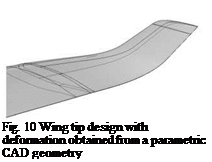
However, mesh deformation conserves the grid topology and small geometry variations produce small mesh deformations in a continuous way. Utilizing this, comparisons of aerodynamic coefficients are better possible and thus uncertainties otherwise introduced by changes of grid topology are minimized. Mesh deformation with FSDeformation was here successfully applied to a shape design change for a wing-tip (figure 9).

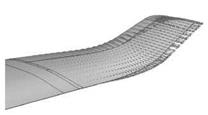
The discrete deformation field was obtained from the parametric CAD model (CATIA V5) using a two-stage process (first the treatment of curves and then sur­faces). In a predictor step, the deformation field is determined by subtracting points on discretized corresponding CAD curves. This gives an initial surface deforma­tion which may not be accurate on the inner region of surface panels apart from the bounding curves.

Applications

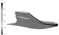
Fig. 9 Wing tip shape design example

Подпись: Fig. 10 Wing tip design with deformation obtained from a parametric CAD geometry
Applications

(a) Parametric CAD geometry (b) Discrete deformation field calculated

from parametric CAD

In the corrector step surface points are projected to the new CAD geometry. The projection vectors together with the displacement vectors of the discretized curves then builds the final discrete deformation field (figure 10(b)). It serves as input for the new tool FSDeformation to accurately move all points of the CFD grid corres­ponding to the parametric change of the CAD geometry.

Interpolation Quality Comparison

The different reduction algorithms in section 4.1 to 4.3 select different base point sets Xs from the input data site set Xinp. This section is comparing the resulting interpolation errors in a test case.

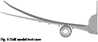
Therefore the extremely deformed half model airplane, as seen in figure 6 is used. The input base points Xmp and their deformation vectors AXmp were calculated with a structural loads program. The tool generates for each surface grid node a deformation vector, so the cardinality of Xmp and AXinp is quite large with a value of ninp = 137,136 for the wing without engine only.

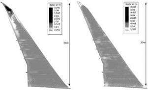
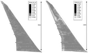
Figure 7 shows the interpolation error ei for the bottom surface of the wing, because it used to show higher interpolation errors. The settings for the interpolation and base point reduction can be seen in table 1.

Because the structural loads tool gives an deformation output for every surface grid node, the interpolation error for the surface nodes e = (ei)i=1 can be cal­

culated by taking the differences between the calculated interpolations AHi and the input deformations Axi:

Єі = \А% – Axi\2. (43)

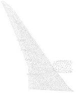
The picture 7(a) clearly shows that the base points, chosen by the equidistant reduction method, are not satisfactory in the outer wing part. The outer 30 percent of the wing show strongly increased error values. This result has motivated to improve the base point selection process. The other reduction algorithms show a strongly improved interpolation error in this part of the wing, too. The mean absolute error ё of each test case for the actual 2000 base point setting, and additionally for another test series with only 1000 base points is given in table 2. Furthermore, this table contains the variance Var (e) and the maximal error max(ei).

i

The table confirms the impression of the given plots: All new methods choose base points resulting in a significantly lower interpolation error. Furthermore, the variance Var(-) indicates that less fluctuations in the error can be expected. The maximum error is lowered by up to 92 percent.

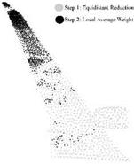
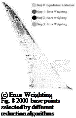
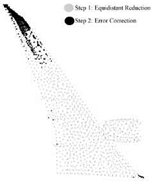
Figure 8 shows how the base points are chosen by the different algorithms. The equidistant reduction algorithm (7(a)) distributes the base points nicely over the whole domain. Taking a closer look, the decreased density of points in the thin parts of the wing, like the trailing edge and the tip, can be recognized.

Table 1 Test settings

Reduction method

Parameter

RBF ф

Equidistant reduction

Wendland’s C°, impact radius r = 20.0

Local average weighting

fracequi = 0.5, dmin — dmaxiЮ

Error weighting

fraCeqm = 0.5, ^EWSteps = 3

Error correction

fracequi = 0.5

(a) Equidistant Reduction


(b) Local Average Weighting


Interpolation Quality Comparison

Interpolation Quality ComparisonInterpolation Quality Comparison

Table 2 Test results interpolation error e = (et)= n.

(a) 1000 base points

Reduction method

e [m]

Var(e) [m1]

max(<?/) [m] І

Equidistant reduction

5.30E-03

8.52E-02

1.24E-04

Local average weighting

1.56E-03

3.87E-02

3.83E-06

Error weighting

1.52E-03

1.10E-02

3.00E-06

Error correction

1.40E-03

8.99E-03

1.19E-06

(b) 2000 base points

Reduction method

e [m]

Var(e) [m2]

max (в/) [m] і

Equidistant reduction

2.33E-03

2.52E-05

4.99E-02

Local average weighting

8.60E-04

1.92E-06

1.91E-02

Error weighting

6.86E-04

6.20E-07

7.92E-03

Error correction

7.38E-04

4.55E-07

3.83E-03

Interpolation Quality ComparisonInterpolation Quality Comparison

Подпись: (c) Error Weighting Fig. 8 2000 base points selected by different reduction algorithms Interpolation Quality Comparison

(a) Equidistant Reduction (b) Local Average Weighting

The new methods have all used the equidistant reduction algorithm in the first step for half of their base points. The remaining half has been selected differently, besides all algorithms concentrate the selected points in the outer wing part.

The local average method (8(b)) is the most extreme example for this behavior. Because the deformations are increasing with a parabolic character, the weights used to be more significant in the outer part. Supplementary, the more narrow getting wing supports this behavior, because the neighborhood of a certain point would contain more points of the side closer to the fuselage then from the outer side, which influences the local mean deformation.

The two remaining approaches based on the interpolation error are choosing their base points similarly. A difference between the error based greedy algorithms is that the error weighting algorithm is distributing the points more numerous in areas far away from the outer wing. The error correction algorithm has selected most points in the tip area.

The results show the best point selection for the error weighting and error cor­rection method. But one has to keep in mind that error correction is only working with radial basis functions with limited influence range, while error weighting has the larger computational costs (7 times larger than error correction).

Error Correction

The error correction algorithm was originally presented in [2, p. 7]. The algorithm tries to correct the а-interpolation coefficient vector locally. Therefore, unlike the previous methods, it is not using the interpolation approach including a polynomial (9), but instead the basic approach without an added polynomial (5):

n

s(x) — Хаіф (l|x-x;||) • (36)

i— 1

Furthermore, the coefficients а; are not calculated by inverting the interpolation matrix A, but instead by correcting them during the iterations continuously. In each step the interpolation error e;, і — 1 ,••, nmp of all deformation vectors

AX — { AXb Ax2,…,AXninp} (37)

at the data sites

Xinp — ^ xinp, 17 xinp!2,—7 xinp, nin^ (38)

is recalculated. The coefficients

а — (аі)І—1,:ППр (39)

and the deformation vectors Axxi are adjusted locally by the radial basis function belonging to the base point with the largest interpolation error eiworst — ||dAxiworst ||2. The correction of aiworst is performed by

^OJr’worst ф ^Q) ^^’iworst; (40)

which is used to update the interpolation values of all base points by

Axi — Axi + A aiworst Ф ( IlXi – xiworst II 2) (41)

In every step in equation (41) the error eiworst at of the deformation Axiworst is changed to zero, since

Подпись: Ax,

(42)

Error Correction

But the corrections for the deformation vectors AX*, which are located inside the impact area of the base point xiworst, are not necessarily decreasing the interpola­tion error. Hence, if fts, max > «inp base points should be selected, the algorithm will run infinitely without reducing the interpolation error to zero. Additionally, the al­gorithm "tends to show a degree of self limiting behavior in terms of how many points it uses ([…]), often returning to correct a previously identified point rather than introducing a new one" [2, p. 8].

The paper [2] uses the algorithm above to approximate the coefficients ai of equation (36), but also recommends not to use these coefficients. Instead the selected base points in Xs should be used for exact interpolation, which uses the inversion of the interpolation matrix as seen in section 2.1.1. The algorithm implemented into the deformation module presented in this document uses this recommendation and, secondly, instead of the interpolation approach (36) the approach including a polynomial as seen in equation (8) for the interpolation matrix creation.

Because the results were still not satisfactory, this approach has been combined with an initial equidistant reduction step to choose fracequi • ns, max base points by the algorithm presented in section 4.1.

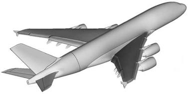
Подпись: Fig. 6 Half model test case
A big disadvantage of the algorithm is that it only works with radial basis func­tions ф (r) with the maximal value for r = 0, so radial basis functions with local influence range.

Weighting by Interpolation Error

The algorithm presented in this section is combining the approach of the weighted distance reduction with the interpolation error calculated for the input data locations. In this case, the distance weights

W = {W1, W2Winp} (33)

are equal to the error of interpolated deformation vectors AXinp.

The basic scheme of the algorithm looks like:

• Select start base point set Xs with corresponding deformation vectors AXs by equidistant reduction

• Do nEWSteps times:

– Interpolate deformations at input points X^p, by using the sets Xs and AXs, to get the deformation vectors AXinp

– Calculate weights Wi by comparing AXmp to AXinp

– Add further base points and deformation vectors by weighted distance reduc­tion to Xs and AXs, respectively.

The type of greedy algorithm, which recalculates the exact interpolation error in each step, is also proposed in [2, p.9].

To interpolate the input points X^p in each step, a new interpolation matrix Hk has to be created from the already chosen base points Xs and inverted in every iteration step. Then the error can be calculated by interpolating the deformation vectors AXs of these base points to the input set Xinp to get the interpolated data set
and taking the pairwise difference to the input deformation vector set AXmp to com­pute the weights

Подпись: (35)wi — ||Axmp, i Axmp, i||27 i — 1 2:-": ninp.

Weighting by the Difference to the Local Average Deformation

This weighting approach takes the deformation vectors Axinpii into account directly. It uses a function FindNeighbours (x, X, AX, d), which returns subsets of

less than d to x. In this case the distances are not weighted yet. The weights for the input point xinp, i are then calculated by

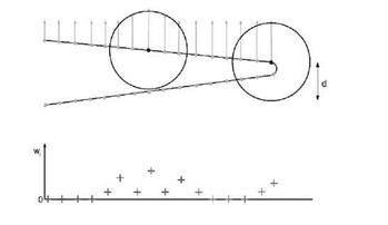
The idea is to develop an expression that favors the base points, the absolute de­formation value of which is different to the average deformation value А. тпь of its neighbors. Another thought is that the nodes at the outer tips of a deforming body will get a higher weight, since at the tip the deformations reach usually their max­imum and consequently differ strongly from the neighborhood mean. An approach which only takes the gradient into account would not result in a higher weight for the outer base points, because the deformation gradient would not have a peak at an outer base point. An example to illustrate this idea can be seen in figure 5. This simplified example shows why the approach leads to higher weights for the base points on the tip, the deformation vectors of which should not be neglected in the final base point set. It shows a tip body with a slight rotational deformation. The deformation vector with the largest value is on the tip of the body. The equidistant reduction algorithm from section 4.1 could easily fail to select the maximum de­formation vectors. Because of the higher weight values at the tip this would happen less likely with the new algorithm.

This example shows a disadvantage of the algorithm as well. If the gradient of the deformation vectors is constant in a certain area, the weights will tend to zero. This will lead to a very low base point density in the next step. To get a lower border for the density, the final reduction method is combined with the equidistant reduction method. First a fraction fracequi of the desired ns, max base points is chosen by the equidistant algorithm, then the remaining base points and deformation vectors are selected with the weighted distance approach.

Weighting by the Difference to the Local Average Deformation

Fig. 5 Schematic example for weights w of the upper base points with their deformation vectors