Category NEW DESIGN CONCEPTS FOR HIGH SPEED AIR TRANSPORT

16.5.1 Oblique Flying Wing

The design presented here is part of a MIDAS design cycle described previously in paper (354). The global design was optimized for a Mach number of 1.6 and therefore had a fixed wing plan – form. sweep and thickness distribution. In the global model a preliminary wing planform was de­termined. and the assumption was made that there existed a thickness and camber distribution which would produce a lift-to-drag ratio of 11 at Mach 1.6 with a cruise lift coefficient of 0.10. This globally optimized aircraft had a span of 120m and a 14.2 m w ide center section chord that was 2.7 m thick. It was assumed that near elliptic off design load distributions could be obtained by unsweeping the wing at lower Mach numbers and deflecting the trailing edge suitably. It is therefore acceptable to just optimize the aircraft with respect to cruise drag while keeping the span, and the center section (passenger cabin) dimensions the same.

The objective of the aerodynamic shape optimization is to find the best aerodynamic shape (minimum drag) under these constraints and compare it with the value projected by the global model. In this detailed geometric shape optimization we must therefore derive a shape that does not interfere with and enables the assumptions of the multidisciplinary global optimum The global optimum was defined with respect to total operating costs.

The design variables were:

1. Angle of attack a and continuously varying section incidences expressed as a Taylor series afe/ у ■* CjV2 *cj y*+c4 y4)

2. Wing bend expressed as a Taylor scries zfc/y-fcjy^+cjУ*+с4у4). The z curvature produces an anti-symmetric twist distribution when the wing is obliquely swept.

3. Outboard wing chord(y) at 25. 40 and 60 m (tip). The wing chord distribution is assumed to be symmetric between left and right side (all у cuts arc mirrored) and is assumed to vary lin­early between the defined у cuts.

4. cruise sweep A was variable but limited to 70 degrees.

5. Wing shape functions expressed as fourth order Taylor scries Y; {stfcіУ+С})^+c+c4y4}

ТІю constraints were:

1. The cruise lift coefficient C{ <0.1

2. No pitching and rolling moments around 32 root chord c. g.

3. Normal Mach numbers on the wing greater than 0.4 to prevent trailing edge separation. Nor­mal Mach numbers not greater than 1.1 to prevent strong nonlinear effects that are not ac­counted for in the linear potential code.

4. Aisles higher than 2.2 m. cabin doors higher than 1.95 m. cargo hold higher than 1.7 m and underfloor crash zone higher than 50 cm. An extra 10 cm is reserved on each side of the ge­ometry for structural reinforcements This corresponds to current Airbus standards. Including structural dimensions this resulted in a maximum external thickness of 2.70 m.

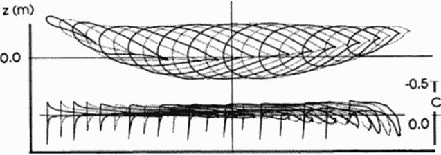
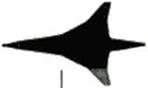
Figure 93 shows the optimized design. Remarkable is the wing bend that the optimizer applied to create an elliptic lift distribution Wing bend has the same effect as twist, but as the wing unsweeps, bend docs not produce an asymmetric loading. In comparison to earlier designs by the author based on inverse methods (350) the current designs are much more symmetric and have flatter pressure distributions. The current design also achieves near the minimum theoreti­cal drag at supersonic flow. It achieved the projected lift-to-drag ratio of 11 very accurately and therefore validated the overall approach. The kink in the 3rd section from the left is not caused by the shape functions, but by the kink in the planform. The sections and pressure distributions shown in Figure 93 are streamwisc slices of the oblique flying wing.

50 I M=1.6CL=0.1

-60.0 o. o 6o. o

x Cm)

Figure 93 Optimized Oblique Flying Wing

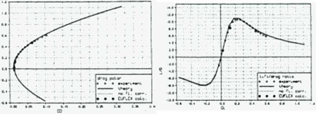
A linear panel code with real flow corrections was used to analyze drag for 3D supersonic wing body configurations. This analysis code was developed by the author from Woodward’s wing – body code (3551. anti solves the linear Prandtl-Glaucrt equation for a thin panel geometry. The power plants are modeled as stream tubes that displace ambient fluid and therefore cause wave drag. Friction is calculated stnpwise over the cursed geometry assuming a fully turbulent bound­ary layer. No effort was made to couple the boundary layer equation to the potential flow pressure distribution. Potential drag is calculated with surface integration and a calculated value of the leading edge thrust. The correct leading edge thrust is found by combining the far-ficld drag as calculated by the Lomax supersonic area rule (345) and Trefftz-plane integration. The leading edge suction is then corrected for real flow effects using the method of Carlson (335|. The Toren – bcck quasi-empiric method (348] is used to model the effect of flap deflection. An overview of this method is given in Figure 91. A more detailed description can be found in the author’s thesis

(350) .

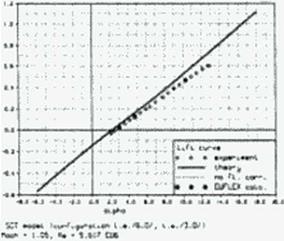
The forces and moments calculated with this method compare well with values meas­ured from the NASA Ames Oblique Wing development program, a generic SCT, a generic fight­er and the Munroe NASA arrow wing tests. Figure 92 shows the calculated and measured forces and moments for a generic SCT with 12 degrees leading and 3 degrees trailing edge flap deflec­tion at Mach 1.05—a difficult case for panel calculations. Our method, which was applied to a panel half-model with a resolution of no more than 120 panels, look one second per flow point on our workstations. The Euler method EUFLEX (343) with a decoupled boundary layer calcu­lation took about an hour on a Cray.

non-linear corrections

forces, moments

Figure 91 A panel method with flow corrections to evaluate forces.

The type and number of constraints are highly problem-dependent. Typical constraints for com­mercial wing designs arc:

• Lift and angle of attack. Either the lift C{ or angle of attack a are constrained or defined as input values. For the horizontal tail plane, both can be simultaneously constrained.

• Minimum and maximum lift. Maximum lift at low speed (=» 50m/s) C{ for a given Rey­nolds number influences takeoff and landing performance and is therefore an important pa­rameter. For horizontal tails, the minimum lift at low speed C. is an important constraint.

Ljmn

For slender supersonic aircraft the maximum lift is usually defined by a maximum angle of attack of 20°. according to the ‘Concorde’ SST regulations.

• Buffet onset at 1.3g relative to Ig cruise. Although a buffet onset is difficult to predict exactly, a conservative estimate can be made using the trailing edge separation criterion [340| based on trailing edge pressure coefficients. Buffet of this type is usually a problem for transonic wing designs.

• Pitching moment C. This is usually not particularly important for subsonic transports but is a major issue for supersonic transports The hinge moment ^ is an important constraint in the design of control surfaces.

• The aircraft thrust must be at least equal to the drag also at off-design points, of which the most critical are usually at the high lift and high Mach number comer of the envelope. The allowed drag creep as a function of Mach number or lift is also often constrained.

• Geometry. The airfoil thickness and thickness distribution are usually subject to structural and geometric constraints such as spar depths.

• Engine installation. The wing design should take into account the disturbances due to engine installation. This is done implicitly by including the engine in – and outflow with the nacelle in the drag balance. When a surface (such as a wing) is placed near a nacelle it will then as­sume a shape such that the drag is minimized (e g. interference minimized)

The variables of our problem describe the aerodynamic shape of the aircraft. Over the last two decades, many engineers have tried to describe the shape of a wing accurately with only a few parameters while maintaining flexibility. There arc three general classes of aerodynamic shape functions:

• Linear combination of existing wing sections. This geometric approach to the airfoil design problem is a derivative of the original NACA method {330}. Although this method is compu­tationally efficient, at DA this method has often given only trivial solutions (c. g. the old air­foil) due to the low flexibility inherent to this geometrical representation. In addition, there is little physical foundation for the implicit assumption that the drag (objective! of a linear combination of airfoil geometries is linearly or at all related to the drag of the individual air­foils.

• Analytical shape functions arc linearly superimposed to define a wing geometry. Examples Of these include Hieks-Hcnnc functions. Wagner functions and the patched polynomials dis­cussed in reference 1344j. as well as the Legendre polynomials used by Reneaux (346J and

the splines used by Coscntino (336]. Unfortunately, the number of parameters required for these shape functions arc usually too high to allow multipoint three-dimensional design. Eve­ry lime, a minimum of 30-40 points arc required to define each airfoil. Even if only five air­foils are sufficient for defining a wing, about 200 parameters will be necessary. This number of variables is simply too great for practical optimization at present. Coscntino optimizes a 3D wing by allowing variations over only a small portion of the wing. Lee has proposed patched polynomials as a way of flcxiblcly modeling an airfoil section with only sixteen pa­rameters. Although this approach does produce a flexible geometry, the performance of the sections designed with this method cannot compete with those produced by experienced en­gineers using inverse methods.

• Special aero-functions were proposed by Rcncaux [346] for designing airfoils with a mini­mum number of parameters. This approach automates the steps that an expenenced designer follows when using an inverse method. ‘Good* pressure distribution types are defined, along with the shape or special aero-functions that produce these pressure distributions. Unfortu­nately. for a given pressure distribution type, these aero-functions vary with Mach number, and this method is therefore impractical for multipoint designs. This method has all the dis­advantages of inverse methods discussed in the Introduction.

At DA (352) the author has introduced another type of function, a highly nonlinear spe­cial aero-function, which can optimize the shape of a 3D wing with adequate flexibility using current computer technology. It is now being used for the industrial design of transonic and su­personic wings. Its application will be shown in the next section. These shape functions produce the aircraft geometry in any resolution.

Multipoint aerodynamic optimization can generally he described in the form of reference (353|:

I. Select objective function.

2. Select variables and constraints.

3. Select optimizers).

4. Optimize and analyze the results.

16.3.1 Drag as an Objective Function

Consider the objective function О described by the total energy loss due to aircraft drag during the operation of the aircraft over n missions:

In this expression./^ is the probability of mission i. and r is the block range for that mis­sion. This expression can be simplified by weighing the drag over a number of representative de­sign points:

m

о = X и’.со (107)

I В I

In our experience, five design points are enough to describe a multipoint design ade­quately.

A. Van dcr Velden
Synaps Inc.. Atlanta, GA, USA

16.1 Abstract

This paper will discuss examples of supersonic aerodynamic shape optimization as developed for Daimler-Benz Aerospace Airbus by Synaps. Inc,

First, we will introduce a general approach to aerodynamic shape design based on min­imization of energy consumption during aircraft life while considenng realistic constraints on lift, pitching and rolling moments and geometric dimensions. The analysis is performed using a potential code with real flow corrections and a decoupled boundary layer calculation. Finally, this method is applied to the design of the European Supersonic Civil Transport and the Oblique Flying Wing.

16.2 Introduction

Engineers have long sought to improve wing design methods Initially, simple geometric shape functions were used to characterize airfoil shapes, the NACA airfoil classification system using this method is described in reference [3301. Unfortunately these NACA airfoils had high drag at transonic speeds, and therefore more refined shapes with reduced (or not transonic shocks were required. More recently, successful transonic wings have been designed by defining a (nearly) shock-free transonic pressure distribution and using an inverse solver to find the corresponding airfoil geometry Though such methods can be applied in high-transonic flow, in supersonic flow

these methods loose their meaning because the optimal pressure distribution cannot be shock­less.

During the days of Concorde and the SST, methods not based on pressure distributions were introduced to solve supersonic aircraft design problems. These methods arc still in use to­day. A good overview paper on these methods was written by Baals, Robins and Harris 1331]. The method first area-rules the fuselage wing combination. The wing lift distribution is opti­mized with Langrangc’s method of undetermined multipliers 1349J(334| for minimum drag. This optimum lift distribution can then be inverted into the geometry using linear theory. But often, the wing shapes derived from such inverse methods exhibit camber kinks due to ill conditioned aerodynamic matrices that require post processing. Variations in the wing planform can also not be considered since it would require a recompuution of the aerodynamic matrices.

A solution that can be used for both transonic and supersonic flow was proposed by VandcrPlaats and Hicks (341). They applied numerical optimization techniques combined with a nonlinear flow analysis methods such as Euler to modify a wing shape such that an arbitrary objective function representing the design goals could be minimized. Although their work was done twenty years ago, computer speeds have MM increased sufficiently to make it practical with the shape functions they proposed. Recently Hicks. Reuther and Jameson have applied this tech­nique on supersonic wing body combinations using the Euler equations.

Since the underlying potential flow theory has appeared to work very well for prelimi­nary supersonic aircraft design, most manufacturers therefore sec no need to change to compu­tationally more expensive and less tested methods at this time. Another advantage of potential flow cited by some engineers involved in the ESCT project, was the inherent separation of wave drag, induced drag and friction drag. This separation of drag components helped to analyze prob­lem spots and the low computational effort reduced the critical design turn around time Though the author agrees with this view, the design method as practiced today is cumbersome and in­flexible as to the use of constraints and modeling of new types of configurations.

The current industrial supersonic wing design methods typically do not include leading edge suction criteria or vortex development Both phenomena influence the forces and moments significantly, especially at subsonic speeds.

This paper combines the direct numerical optimization of a completely flexible wing- body-nacelle configuration w ith an industrial potential flow code with corrections.

Any MIDO algorithm stresses high transportability as well as extensive graphical user interac­tion and support. The product is a full featured, self-configuring MIDO package capable of uti­lizing a variable number of diverse CPU’s and input/outpul devices that is valuable to research and industrial practical use. Massively parallel machines arc the latest significant step in this technology. Tins expansion from a single CPU has greatly increased computational power; how­ever, it lus also increased the problem of transportability of the software. The rationale behind the advent of FORTRAN 90 was that users needed a standard method for the utilization of a var­iable number of CPU’s. The CPU job tasking, while referred to by the programmer, is essentially handled by the FORTRAN 90 compiler. While FORTRAN 90 delivers a standard to the user of parallel machines, it in no way increases the user’s interface with the code itself. The researcher or design engineer who simply provides a source code to the FORTRAN 90 compiler has no standard method for producing runtime graphics, real-time flow-field visualization, or other graphical user interactions. The only option for the user is to make calls to an external graphics package that is loaded on the particular system in use. By doing this, (he generality of the code is lost. This problem is also true of other input/output devices.

This problem can be solved by giving the user real-time graphical visualization as an integral part of the MIDO software package that will allow researchers and design engineers to watch as they analyze and optimize their designs. Furthermore, criteria and boundary condi­tions are dynamic, allowing users to alter or update them as execution progresses. The problem of transportability is overcome because the package does not require a compiler since such MIDO package is prc-compiled and pre-linked. It is a stand-alone executable that detects and utilizes the host system. It is a self-contained, auto-configuring package that is to aerodynamic shape design and thermal design what I DEAS and GENESIS arc to structural design An exe­cutable such as this MIDO package, can also be developed in lower level languages such as С/ C++ or Assembler rather than less efficient high level languages such as FORTRAN. As well as being more efficient, low level languages operate in a regime that is close to tlie native language of the machine, allow ing direct manipulation of the host system hardware This direct access programming allows the final product to he highly modular and adaptable. These advantages could be utilized in the MIDO package with the end result that the user can choose the desired aspects of the package, and the algorithm will conform itself.

Because of the complex algorithms and high degree of programming skills required for this package, the development process can be divided in two stages.

During the first stage of such a MIDO package development, it can be written in FOR­TRAN 77 so that its legitimacy can be checked. Numerical solutions produced by this package can be checked against available analytical and experimental data to ensure that true physical phenomena are captured. Then, the MIDO package can be rewritten into low level languages as rmnlules to a central-switching logic that is designed for a single CPU system. A full-featured interactive graphical environment can be developed for this system.

The second stage of the suggested MIDO package development can be centered on the expansion of the package to include support for a variable CPU system. Package development can culminate in its high modularity, full user interface environment (for a PC with MS-Win – dows-LINUX and workstations with UNIX and X-Windows), ability to change How solvers in the environment, change boundary conditions, switch between analysis mode, inverse design mode, and optimization (based on user defined criteria) mode in the environment while devel­oping a desired design

Although most aerodynamic, heat transfer and elasticity analysis codes are written in FORTRAN while genetic algorithms and graphical interfaces are more efficient when coded in C++ language, the use the PVM (Parallel Virtual Machine) or the new generation MPL (Mes­sage Passing Libraries) can make their simultaneous use possible. With the PVM or MPL. the hybrid GA optimizer can be compiled from a C++ source, while an analysis code can be com­piled from a FORTRAN source. The message-passing between the two running codes is not extensive, yet it is independent of the language of the source code.

The efforts should be focused in developing a commercial quality MIDO package for research and direct industrial use. Algorithms should be modified to run in FORTRAN 90 on parallel CM-2, CM-5. IBM SP-2. CRAY-90, etc. or clusters of arbitrary PC’s. w4*rkstations and

mainframes connected through a router thus stressing transportability to an arbitrary number of CPU’s.

15.2 Conclusions

The Multidisciplinary Inverse Design and Optimization (MlDO) approach to a complete aircraft system design is already a reality in some of the leading companies. It has been taking two dis­tinct paths where cither a semi-sequential disciplinary optimization is performed or a simultane­ous analysis and optimization of the entire system is performed Both approaches have their own difficulties with computing time requirements and numerical stability. These issues will progres­sively be resolved by a better use of massively and distributed parallel computation and by the development of faster iterative algorithms for analysis and constrained optimization.

The treatment of complex geometries has led us to adopt a multi-block grid made of several structures w ith overlapping or patched domains. The method of distributing domains over proc­essors is important in that it leads to typical load balancing problems and synchronization of waiting time. Issues that need to be addressed are: flexibility in load balancing, reading and gen­erating block data, reading and generating interface data, and updating block and interface data during communication. The advantage in using the multi-block approach is that one can have more than one block solver (for example. Euler. Navier-Stokes. etc.) in different blocks depend­ing on the complexity of the flow field in a given block, thereby improving the overall efficiency of the algorithm. The most important parallelization issue for CFD applications is the way in which the computational domain is partitioned among a cluster of processors. Even a highly ef­ficient parallel algorithm can give poor results for a poorly implemented domain decomposition The domain decomposition technique has been successfully implemented on both SIMD and dis­tributed memory M1MD computers. Algorithms like the ‘Masked Multi-block Algorithm" allow for dynamically partitioning the domain depending on the distnbution of load among processors. This eliminates the possibility of distributing each domain on a processor since in most cases do­mains will have irregular sizes. Other algorithms distribute separated planes of a 3-D computa­tional domain between processors to synchronize lime waiting. The measure of the efficiency of a parallel algorithm is given by the ratio of the computation lime to the communication time for a particular application. High performance message passing can be achieved by "overlapping communication", performing assembly-coded gather-scatter operations. A machine like the CM – 2 is a SIMD type machine where most of the parallelization is earned out by the compiler which is responsible for data layout. The Cray’s parallel processing capabilities can be exploited by the use of "auto-tasking" wherein the user indicates points of potential parallelism in the implemen­tation by the use of directives which instruct a pre-processor to reconfigure the source program in such a way so as to enable maximum speedup to be obtained.

An alternative to parallel hardware architecture is the poor man’s machine or PVM (Parallel Virtual Machine) that can simulate a parallel machine across a host of senal machines The programming model supported by PVM is distributed memory multi-processing w ith low level message passing. A PVM application essentially uses routines in the PVM to do message passing, process control and automatic data conversion. A special process runs on each node (each machine) of the virtual machine and provides communication support and process con­trol. However since message passing is carried out on the Ethernet it is considerably slower than the Intel Interprocessor network. There is also an overhead on account differences between speeds of different machines that create load balancing problems.

At present, it is possible to solve an impressive array of complex fluid dynamic problems by nu­merical techniques, but in many instances a minor change in the problem being computed can require an unwarranted amount of operator intervention, and/or an unexpectedly large increase in computer time For example, a minor change in geometry or grid spacing sometimes has a ma­jor effect on convergence and can even lead to divergence, while coaxing a new problem through to a successfully converged solution can take many hours for even an experienced numerical an­alyst. Difficulties of this nature frequently dominate the cost of completing numerical solutions and can prevent the effective implementation of numerical techniques in design procedures.

Reduction of total computing time required by iterative algorithms for numerical inte­gration of Navier-Stokes equations for 3-D. compressible, turbulent flows w ith heat transfer is an important aspect of making the existing and future analysis and inverse design codes widely acceptable as main components of optimization design tools. Reliability of analysis and design codes is an equally important item especially when varying input parameters over a wide range of values. Although a variety of methods have been tried, it remains one of the most challenging tasks to develop and extensively verify new concepts that will guarantee substantial reduction of computing lime over a wide range of gnd qualities (clustering, skewness, etc.), flow field parameters (Mach numbers. Reynolds numbers, etc ), types and sizes of systems of partial dif­ferential equations (elliptic, parabolic, hyperbolic, etc ). While a number of methods are capable of reducing the total number of iterations required to reach the converged solution, they require more time per iteration so that the effective reduction in the total computing lime is often negli­gible.

The existing techniques for convergence acceleration arc known to have certain draw – backs. Specifically, residual smoothing [3011, although simple to implement, is a highly unreli­able method, because it can offer either substantial reduction of number of iterations or и can abruptly diverge due to a poor choice of smoothing parameters (302]. Enthalpy damping (3011 assumes constant total enthalpy which is incompatible with viscous flows including heat trans­fer. Multigridding in 3-D space is only marginally stable [303J when applied to non-smooth and non-orthogonal grids. GMRES method [304] based on conjugate gradients requires a large number of solutions to be stored per each cycle which is iniractablc in 3-D viscous flow compu­tations. Power method (305) which is practically identical to the GNI-MR method 1306] works well w ith a multigrid code. Without multigridding. it is highly questionable if the power method would offer any acceleration when applied to a sy stem of nonlinear partial differential equa­tions. Despite the multigrid method’s superior capability of effectively reducing low and high frequency errors yielding impressive convergence rates, its efficiency is significantly reduced on a highly-clustered grid (302]. (303] and it is difficult to implement reliably. The precondition­ing methods (3071. although very powerful in alleviating the slow convergence associated with a stiff system for solving the low Mach number compressible flow equations, have not been shown to perform universally well on highly – clustered grids. Distributed Minimal Residual
(DMR) method (308). (309) in its present form has the same problem in transonic range. Numerous other methods have been published that arc considerably more complex, while less reliable and effective.

The main commonality to all of these methods is that they all experience loss of their ability to reduce the computing time on highly-clustered non-orthogonal grids (307). (310| that arc unavoidable for 3-D aerodynamic configurations and high Reynolds number turbulent flows.

Existing iterative algorithms arc based on evaluating a correction. AQ‘. to each of the variables and then adding a certain fraction, to AQ’, of the correction to the present value of the vector of variables. Q’. thus forming the next iterative estimates as

= q’ + u)AQ’ (94)

The optimal value of the relaxation factor, ox can be determined from the condition that the future residual is minimized with respect to ox

Instead, corrections from N consecutive iterations could be saved and added to the present value of the variable in a weighted fashion, where each of the consecutive iterative cor­rections is weighted by its own relaxation factor This is the General Nonlinear Minimal Resid­ual (GNLMR) acceleration method (306). summanzed as

• I r _ r – t. _r – I »- .V – 1 / – Л? – I jOC.

Q – Q * ш SQ * Ы ±Q ♦ …♦« SQ (95)

The optimal values of the relaxation factors, ux can be determined from the condition that the future residual is minimized simultaneously with respect to each of the N values of eo’s.

Now. let us consider an arbitrary system of M partial differential equations. If the GNLMR method is applied to each of the M equations so that each equation has its own sequence of N relaxation factors premultiplying its own N consecutive corrections, this defines the Distributed Minimal Residual (DMR) acceleration method (308). (309) formulated as

Qm’ « Q’h ♦ ♦ <** ‘*?«’♦ – * **ii*’ W,* *1 <97)

The DMR is applied periodically where die number of iterations performed with the basic non-accclcratcd algorithm between two consecutive applications of the DMR is an input parameter. Here. (Os are the iterative relaxation parameters (weight factors) to be calculated and optimized. AQ’s are the corrections computed with the non-accclcratcd iteration scheme. N denotes the total number of consecutive iteration steps combined when evaluating the optimum (O s, and M stands for the total number of equations in die system that is being iteratively solved.

The DMR method calculates optimum w’s to minimize the L*2 norm of the future residua! of the system integrated over the entire domain. D. The present formulation of the DMR uses the same values of the N x M optimized relaxation parameters at every gnd point, although different parts of the flow field converge at different rates.

An arbitrary system of partial differential equations governing an unsteady process can be written as К m JjQ я L(Q), where Q is the vector of solution variables, t is the physical time. L is the differential operator and R is the residual vector.

Sensitivity-Based Minimum Residual (SBMR) method (311), (312) uses the fact that the future residual at a grid point depends upon the changes in Q at the neighboring gnd points used in the local finite difference approximation. The sensitivities are determined by taking par­tial dcnvativcs of the finite difference approximation of Rr (r=l……………………………………………………………………………………………….. rmax where rmax is the

number of equations in the system) with respect to each component of Qmt (m = I…., M where

M is the number of unknowns; s = l…………… S where S is the number of surrounding gnd points

directly involved in the local discretization scheme) This information is (hen utilized to effec­tively extrapolate Q so as to minimize the future residual. R Nine grid points located at (і-1J-1; i-lj; i-1. j-fl; ij-1; ij; ij+l; i+lj-l; i+lj; i+l. j+l) arc used to formulate the global SBMR method for a two-dimensional problem when using central differencing compared to nineteen grid points for з three-dimensional case when using central differencing This approach is dif­ferent from the DMR (308). (309) method where the analytical form of R was differentiated

Suppose that we are performing an iterative solution of an arbitrary evolutionary sys­tem using an arbitrary iteration algorithm. Suppose we know the solution vectors Q1 and Q“n at iteration levels t and t+n. respectively. Here, n is the number of regular iterations performed by the original non-accclcrated algorithm. Then. AQ between the two iteration lewis is defined as

Q1 = Q1 + AQ if no acceleration algorithm is used. Using the first two terms of a Taylor senes expansion in the artificial (iterating) time direction, the residual for each of the equations in tlic system after n iterations is

Nonce that the total number of equations in the system is the same as the total number of unknown components of Q. that is. rmax r M. If we introduce convergence rate acceleration coefficients a|. os с*ц multiplying corrections respectively, then each component.

Qm s ’> * . of the future solution vector at the grid point, s. can be extrapolated as

This can be applied at every grid point in the domain, but it results in a huge system of imax x jmax x kmax x M unknown acceleration coefficients, a If each of the a’s is assumed to have the same value over the entire domain. D. the number of unknown a s is reduced to M. This pragmatic approach is called the global SBMR method 1311J. [312J. It requires solution of a much smaller M x M matrix. The future residual at the iteration level (t+n)+1 can. therefore, be approximated by

Subtracting (94) from (96) yields

ці’ **>♦ I

where

(102)

The optimum a’* arc determined such ihat Uk sum of die L-2 norm of the future resid­uals over the entire domain. D. will be minimized.

for m = With the help of (101) and (102). the system (103) becomes

In equation (101)* the R’s and a’s arc known from the preceding iteration levels. Since each am is assumed to have the same value over the entire computational domain, equation (104) gives a tractable system of M simultaneous algebraic equations for M optimum ot|. a2………………………………………………………………………………………

«М

t) (105)

For the general case of a system composed of M partial differential equations with M unknowns, the system (105) will become a full M x M symmetric matrix for M unknown opti­mum a’s.

It is plausible that for non-uniform computational grids and rapidly varying dependent variables, optimum a’s should not necessarily be the same over the whole computational domain. A modification of the SBMR method called Line Sensitivity-Based Minimal Residual (LSBMR > method was developed (311]. (312] to allow a’s to have different values from one grid line to another. The resulting system has. for example, jmax x M unknown a’s. which is quite tractable, although it is more complex to implement than the SBMR method.

The performance of the SBMR and the LSBMR methods (ЗІ I). (312} depends on how frequently these methods arc applied during the basic iteration process and on the number of iterations performed with the basic iterative algorithm that arc involved in the evaluation of the change of the solution vector. In the case of two-dimensional incompressible viscous flows without severe pressure gradient, the SBMR and LSBMR methods significantly accelerate the convergence of iterative procedure on clustered grids with the LSBMR method becoming more efficient as grids are becoming highly clustered The SBMR and the LSBMR methods tested for a two-dimensional incompressible laminar flow maintain the fast convergence for highly non- orthogonal grids and for flows w’ith closed and open flow separation The SBMR method is capable of accelerating the convergence of inviscid. low Mach number, compressible flows where the system is very stiff. An Alternating Plane Sensitivity-Based Minimal Residual (APSBMR) method (312]. a three-dimensional analogy of the LSBMR method, has been shown to successfully reduce the computational effort by 509f when solving a three-dimensional, lam­inar flow through a straight duct without flow separation.

The general formulation of these acceleration methods is applicable to any iteration scheme (explicit or implicit) as the basic iteration algorithm. Hence, it should be possible to apply these convergence acceleration methods in conjunction with the other iteration algonthms
and with other acceleration methods (preconditioning (307). multigndding (310), etc.) to explore the possibilities for a cumulative convergence acceleration effect.

In the case of optimization methods based on sensitivity analysis, live main difficulty is to make the evaluation of the derivatives less difficult and more reliable. A worthwhile effort is to research further on use of the automatic differentiation (ADIFORj based on a chain-rule for evaluating the derivatives of the functions defined by flow analysis code with respect to its input variables [313|-(317). This approach still needs to be made more computationally efficient. One obvious possibility is to utilize parallel computer architecture in the optimization process not only with the gradient search algorithms 13181, (319]. but especially with genetic evolution algorithms (320) where massively parallel approach should offer impressive reductions in com­puting time. The use of parallel computing will become unavoidable as the scope of optimiza­tion becomes multi objective (321|-(325).

An equally worthwhile effort is to further research the "one shot" method that carefully combines the adjoint operator approach and the mullignd method (326]. This algorithm opti­mizes the control variables on coarse grids, thus eliminating costly repetitive flow analysis on fine grids during each optimization cycle The entire shape optimization should be ideally accomplished in one application of the full multigrid flow solver 1326).

Finally, it should be pointed out that although the exploratory efforts in applications of neural networks (327). (328) and virtual reality arc still computationally inefficient, their time is coming inevitably as wc attempt to optimize the complete real aircraft systems. Recent pioneer­ing efforts (3291 in coupling wind tunnel experimental measurements and a muluobjective hybrid genetic optimization algorithm indicate that the decades old dream of effectively and harmoniously utilizing both resources is soon to become a reality.

It is well understood that automatic discretization (boundary-conforming computational grid generation) is the main bottleneck of the entire computational aerodynamics Typically, it takes more time to generate an acceptable new grid for a new realistic 3-D aerodynamic configuration than it takes to predict the 3-D flow field around it. Since any shape inverse design and optimi­zation effort implies repetitive generation of the 3-D grid, it is quite clear that developing a user – friendly, fast and reliable 3-D computational grid generation code is an extremely important is­sue. The existing automatic 3-D grid generation codes accept surface grid coordinates as an input and then generate the coordinates of field grid points. This approach is not reliable in the sense that there is no guarantee that some of the generated grid cells will not fold-over, or become ncc – dlc-likc. or that excessively large cells will not neighbor cxccssivcly-small gnd cells, or that the grid will not be sufficiently clustered in the regions of interest, or dial the grid will not become excessively non-orthogonal. Such problems cause significantly slower convergence of the anal­ysis iterative algorithms, they create significantly larger computational errors, cause numerical instability, and often lead to outright divergence of the iterative process.

Any grid generation algorithm must be computationally efficient in terms of storage and execution time and able to accept even incomplete initial grids, that is. the grids that have only surface grid points resulting from a solid modeling software package (for example. CAT1 A). One technique capable of generating reliable 3-D gnds in an a posteriori fashion is the grid optimization method which has been applied to 2-D [297] and 3-D [298] structured and block-structured [2991 and to 2-D triangular unstructured gnds including automatic solution – adaptive clustering [300). This fully 3-D robust computational grid post-processing algorithm checks the enure onginal grid for possible negative Jacobian* (existence of fold-over grid cells), untangles the gnd lines, and optimizes the grid in a sense that it becomes maximally locally orthogonal and smoothly clustered in the regions of interest.

Notice that this grid generation procedure is especially suitable to the tightly coupled approached mentioned above. In this case, the grid from the flow field smoothly blends with the grid in the solid structure and the interior of the aircraft while clustering at the interface sur­faces.