Category NEW DESIGN CONCEPTS FOR HIGH SPEED AIR TRANSPORT

G. S. Dulikravich

The Pennsylvania State University, University Park, PA, USA

15.1 Introduction

Designing for improved performance and life expectancy of high speed transport configurations is traditionally conducted by performing a repetitive sequence of uncoupled, single-discipline analyses involving flow field, temperature field, stress-strain field, structural dynamics, manu­facturability tradeoffs and a large amount of personal designer’s experience and intuition 1289)- (295|. Since the entire aircraft system is seemingly highly coupled, it would be plausible that both analysis and design should be performed using an entirely new generation of computer codes that solve a huge system of partial differential equations governing aerodynamics, elastodynamics, heat transfer inside the structure, dynamics, manufacturing cost estimates, etc. simultaneously. Tins approach offers very stable computation since all boundary and interfacing conditions arc incorporated implicitly. On the other hand, this approach might not be the most computationally economical since different subsystems (Navicr-Stokes equations, elastodynamic equations, heat conduction equation. Maxwell’s equations, etc.) that form such a complex mathematical system have vastly different eigenvalues and consequently converge at significantly different rates to a steady slate solution. In addition, a rigorous analysis can show that even seemingly highly cou­pled systems arc only loosely coupled and can be analyzed scmi-sequcntially (2%). Such a scmi – scquential approach is presently used by most researchers and the industry since it can utilize most of the existing analysis and inverse design and optimization software as ready and inter­changeable modules with minimum time invested in their modifications, Nevertheless, this ap­proach is much more prone to global instability because of the often unknown and inadequately treated boundary and interface conditions.

In the remaining pan of this article the focus will he on the computational grid, accel­eration of iterative algorithms and parallelization and networking issues that are pertinent to the M1DO efforts.

Another type of inverse problem in elastostatics is to deduce displacements and tractions on sur­faces where such information is unknown or inaccessible, although the geometry of the entire 3- D configuration is given. It is often difficult and even impossible to place strain gauges and take measurements on a particular surface of a solid body cither due to its small size or geometric in­accessibility or because of the severity of the environment on that surface. With our inverse method (281) these unknown elastostatics boundary values can he deduced from additional dis­placement and surface traction measurements made at a finite number of points within the solid or on some other surfaces of the solid. This approach is robust and fast since it is non-iterative. A similar inverse boundary value formulation has been shown (282) to compute meaningful and accurate thermal fields during a single analysis using a straight-forw ard modification to the BEM non-linear heat conduction analysis code. An example of the concept follows using the BEM.

In general elastostatics, we can write for any discretized boundary point V and for each direction T a boundary integral equation (283|

(90)

where the asterisk designates fundamental solutions and the term C| is obtained with some special treatment of the surface integral on the left hand side (283). Explicit calculation of this value can be obtained by augmenting the surface integral over the singularity that occurs when the integral includes the point V. Fortunately, explicit calculation is not necessary as it can be obtained using the ngid body motions The boundary G is discretized into Nip surface panels connected between N nodes. The functions u and p are quadratically distributed over each panel with adjacent panels sharing nodes such that there will be twice as many boundary nodes as there arc surface panels, A transformation from the global (x. y) coordinate system to a localized boundary fitted (^.r|) coordinate system is required in order to numerically integrate each surface integral using Gaussian quadrature The displacements and tractions arc defined in terms of three nodal values and three quadratic interpolation functions. The whole set of bound­ary integral equations can be written in matnx form (ommiting the body forces for simplicity) as

(91)

where the vector! |U| and (PI contain the nodal values of the displacement and trac­tion vectors. Each entry in the (HJ and (G) matrices is developed by properly summing the con­tributions from each numerically integrated surface integral The surface tractions were allowed to he discontinuous between each neighboring surface panel to allow for proper corner treat­ment. The set of boundary integral equations w ill contain a total of 2N equations and 6N nodal values of displacements and surface tractions.

For a well-posed boundary value problem, at least one of the functions, u or p. will be known at each boundary node (either Dirichlct or von Neumann boundary condition) so that the equation set will be composed of 2N unknowns and 2N equations. Since there arc two distinct traction vectors at comer nodes, the boundary conditions applied there should include either two tractions or one displacement and one traction. If only displacements are specified across a corner node, special treatment is required (283).

For an ill-posed boundary value problem, both u and p should be enforced simultane­ously at certain boundary nodes, while either u or p should be enforced at some of the other boundary nodes, and nothing enforced at the remaining boundary nodes. For the simple exam­ple of a quadrilateral plate with four nodes, if at two boundary nodes both u = U and p = P arc known, but at the other two nodes neither u nor p is known, the BEM equation set before any rearrangement appears as

where each of the entries in the |H) and (G) matrices is a 3×3 submatnx in 3-D elasto – statics. Straight-forward algebraic manipulation yields the following set

The right-hand side vector {F) is known and the left-hand side remains in the form (A)(X). Once the matrix (A) is solved, the entire u and p fields within the solid can be easily deduced from the integral formulation. The equation set |A)(X1 = (F) resulting from our inverse boundary value formulation is highly singular and most standard matrix solvers will produce an incorrect solution Singular Value Decomposition (SVD) methods [284] can be used to solve such problems accurately. The number of unknowns m the equation set need not be the same as the number of equations (284), so that virtually any combination of boundary condi­tions will yield at least some solution. Additional equations may be added to the equation set if u measurements are known at locations within the solid in order to enhance the accuracy of the inverse steady boundary condition algorithm. A proper physical solution will be obtained if the number of equations equals or exceeds the number of unknowns If the number of equations is less than the number of unknowns, the SVD method will find one solution, although it does not
necessarily have to he the proper solution from the physical point of view (285]. Thus, the more overspecified data is made available, the more accurate and unique the predicted boundary val­ues will be.

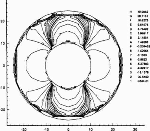
The accuracy of the inverse boundary condition code w as verified (281 ] on simple 2-D geometry consisting of an infinitely long thick-walled pipe subject to an internal gauge pressure. Тік shear modulus for this problem was G = S OxlO4 N/mm: and Poisson’s ratio was v = 0.25. The radius of the inner surface of the pipe was 10 mm and the outer radius was 25 mm The inner and outer boundaries were discretized with 12 quadratic panels each The internal gauge pressure was specified to be Pr = 100 NVmm*. while the outer boundary was specified with a zero surface traction. Figure 88 depicts a contour plot of constant values of stress tensor compo­nents Gyy that was computed using the analysis version of our second-order accurate BEM elas – tostatic code. The numerical results of this well-posed boundary value problem were then used as boundary conditions applied to the following two ill-posed problems.

Figure H8 Contours of constant stress, ayy from the wellposed analysis of an annular pressurized disk.

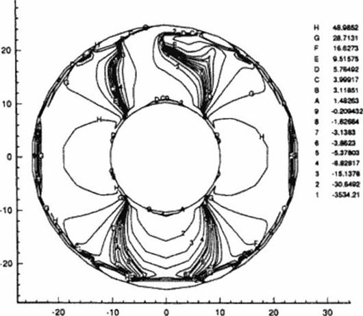
First, the displacement vectors computed on the inner circular boundary were applied as over-specified boundary conditions in addition to the surface tractions already enforced there At the same time nothing was specified on the outer circular boundary. Figure 89 represents the

contour plot of <Jvy that was obtained with our inverse boundary value ВБМ code. This stress averaged a much larger error, about 3.0%. with some asymmetry in the stress field, when com­pared with the analysis results.

Next, the displacement vectors computed on the outer circular boundary by the well – posed numerical analysis were used to over-specify the outer circular boundary. At the same lime nothing was specified on the inner circular boundary. Figure 90 the contour plot of ayy as computed by the inverse ВПМ technique. The predicted inner surface deformations were in error by less than 0.1%. while the predicted inner surface stresses averaged less than a 1.0% error as compared to the analysis results.

It seems that an over-Specified outer boundary produces a more accurate solution than one having an over-specified inner boundary. It was also shown that as the over-specified boundary area or the resolution in the applied boundary conditions was decreased, the amount of over-specified data also decreases, and thus the accuracy of the inverse boundary v alue tech­nique deteriorates.

H 44M52

a «rut f!»un E «51*7»

0 S 76492

c sweir

В 111N1 А 1«Ж В -020*0?

• Ь.’бб*

7 4.1Ш

• 1W23

S 5.27«OJ « IUIV 3 -11137»

1 ЗС54Є2

1 3634.21

-L.

30

14.5 Conclusions

Siructural design of complex 3-D composite structures is possible only by using reliable optimi – zaiion codes. For simpler configurations with smaller numbers of variables it is also possible to use inverse shape design methodologies based on over-specified surface tractions and deforma­tions. Inverse shape design and inverse boundary condition determination can be performed us­ing both BEM and finite clement techniques. Hybrid optimization algorithms [286] that arc based on genetic evolution, simulated annealing, fu/.zy logic and neural networks and that involve man­ufacturing constraints (287]-(288) will be the candidates for active clastodynamic/aeroelastic control of smart structures.

An e last os tat ic problem is well-posed when the geometry of the general 3-D multiply-connected object is known and either displacement vectors, u. or surface traction vectors, p. are specified every where on the surface of the object. The elastostaiic problem becomes ill-posed when either:

a) a part of the object’s geometry is not known, or b) when both u and p arc unknown on certain parts of the surface. Both types of inverse problems can be solved only if additional information is provided. This information should be in the form of over-specified boundary conditions where both u and p are simultaneously provided at least on certain surfaces of the 3-D body.

The inverse determination of locations, sizes and shapes of unknown interior voids subject to overspecified stress-strain outer surface field is a common inverse design problem in elasticity [276)-(279|. The general approach is to formulate a cost function that measures a sum of least squares differences in the surface values of given and computed stresses or deforma­tions for a guessed configuration of voids. This cost function is then minimized using any of the standard optimization algorithms by perturbing the number, sizes, shapes and locations of the guessed voids. Thus, the process is identical to the already described inverse design of coolant How passages subject to over-specified surface thermal conditions 1280]. It should be pointed out that this approach to inverse design of interior cavities and voids can generate interior con­figurations that are potentially non-unique.

G. S. Dulikravich

The Pennsylvania Stale University, University Park. PA, USA

14.1 Introduction

Design of structural components for specified aerodynamic and dynamic loads can be achieved with an extensive use of a reliable and versatile stress-deformation prediction code and a con­strained optimization code. The finite element method (FEM) is the favorite method for structur­al analysis because of its adaptability to complex 3-D structural configurations and the ability to easily account for a point-by-point variation of physical properties of the material. With the re­cent improvements in the sparse matrix solver algorithms, the finite clement techniques arc also becoming competitive with the finite difference techniques in terms of the computer memory and computing time requirements. For relatively smaller problems in elasticity, it is even more ad­vantageous to use boundary clement method (BEM) because it is faster and more reliable since it is non-iterative and it requires only surface discretization.

14.2 Optimization in Elasticity

The field of structural optimization (269J-(273) has a considerably longer history than aerody­namic shape optimization. Almost every textbook on optimization involves examples from linear elastostatics since these types of problems usually result in smooth convex function spaces that have continuous and finite sensitivity derivatives, making them ideal for gradient search optimi­zation. As the geometric complexity and the diversity of materials involved in aerospace struc­tures has increased, so has the demand for a more robust non-gradient search optimization

algorithms. Consequently, the majority of the present-day Structural optimization is performed using different variations of genetic evolution search strategy and a hybrid gradicm/genetic ap­proach (274|, (275). This is quite evident when researching the literature dealing with structures made of composite materials, ceramically coated structures, and smart structures. In the case of smart structures, their “smart" attribute comes from the ability of such materials to respond with a desired degree of deformation to the applied pressure, thermal, electric or magnetic field. This automatic response can be very fast and can be used for active control of the structural shape in the regions exposed to the air flow. This influences the flow field, surface heat transfer and the aerodynamic forces acting on the structure.

Structural optimization is routinely used for the purpose of achieving aeroclastic tai­loring. Since this requires specifications of a large number of constraints in the form of desired local deformations, this application can also be qualified as a de facto inverse structural shape design. The objective is to find the appropriate shape and orientation of each layer of a compos­ite material to be formed so that the final object (for example, a helicopter rotor blade, an air­plane wing, etc.) will have (he most uniform stress distribution (thus minimum weight) and. when loaded, will deform into a desired form.

Since the local values for the convective heat transfer coefficient, on the surfaces of the 3- D coolant flow passages have been specified thus far, it is necessary to compute their actual val­ues. This can be done using a reliable 3-D Navier-Stokes code with the best turbulence model available at the time. With the specified inlet coolant temperature and the already determined temperature distribution on the walls of the coolant flow passages, a single run w ith the Navier – Stokes code should predict a detailed distribution of h^y on the 3-D surfaces of the coolant flow passages.

If the predicted values of h^** are significantly different from those used in the previ­ous tasks, the last two tasks should be repeated until convergence.

13.2 Conclusions

It is possible for thermal design and optimization to perform relatively efficiently, even in a fully 3-D case, if BEM codes arc used for thermal field analysis and inverse determination of unknown boundary conditions and optimization is performed using a hybrid genetic cvolution/gradicnt search constrained optimization algorithm. One specific conjugate heat transfer design and op­timization scenario has been suggested for which all of the individual tasks have been proven to work by the author’s research team. The main uncertainty of the entire conjugate heat transfer design process still rests w ith the issue of reliability of turbulence models in typical 3-D Navicr – Stokes flow-field analysis codes to predict surface temperatures and heat fluxes.

Next, the designer could run a 3-D Navier-Stokes coolant flow analyst!, code and compare its predicted coolant passage wall temperatures with the temperatures obtained in the previous task. The objective could be to minimize the difference in coolant passage surface temperatures ob­tained from the Navier-Stokes coolant flow analysis code and the heal conduction BEM code. This will be achieved by further altering the shapes of the 3-D coolant passages. This iterative modification of the 3-D coolant passages is required since all thermal boundary conditions on the external and internal surfaces must be compatible with each other and with the corresponding flow fields.

In addition, the converged configuration of the 3-D coolant passages might not be desirable from the manufacturing point of view and might not be structurally sound. Thus, the designer should use the converged configuration of the 3-D coolant passages only as an intelli­gent initial guess to help in the structural design. For this purpose the designer might wish to specify the locations of mid-planes of the walls separating the converged shapes of 3-D coolant passages and treat them now as mid-planes of the future intenor struts. Other design constraints and requirements may be considered and incorporated. This automatically defines the initial thickness distnbutions of each strut and the wall. These thicknesses can be parameterized with a small number of (3-splinc coefficients which can then be the design vanablcs in the optimization process

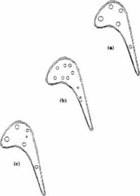
Thermal boundary condition inverse determination В EM codes can than use the hot surface tem­peratures and heat fluxes and non-iterauvely predict the distribution of temperatures and heat fluxes on walls of the coolant passages. Convective heat transfer coefficients can then be com­puted on the walls of the coolant passages. These coefficients might locally exceed the realistic values attainable with the coolant flow in smooth passages. The locally varying heat convection coefficients should, therefore, be limited to their maximum allowable values The corresponding modified heat fluxes on the walls of the coolant passages can then be determined. These "cold" heat fluxes and temperatures will then be submitted to the BEM inverse code that will determine the corresponding “hot* temperatures and heat fluxes. The resulting computed hot surface tem­peratures and heat fluxes will be different from the optimized hot surface values. The difference between the computed and the previously optimized hot surface temperatures and heat fluxes will then serve as the forcing function in a constrained optimization code. It will drive the sizes of unnecessary coolant passages to zero, while relocating, resizing, and reshaping the minimum necessary number of the passages until the differences in the computed and the optimized hot surface heat fluxes and temperatures arc negligible. Minimum allowable distances among the coolant passages or from the thermal bamcr coating interface will serve as constraints (Figure 86 and Figure 87).

As a by-product of the aerodynamic inverse design using Navicr-Stokcs computation of the hot gas flow field (with the specified temperatures as thermal boundary’ conditions on the hot sur­face) the corresponding hot surface heat flux distribution can be obtained. Since one of the global objectives is to minimize the coolant mass flow rate, the total integrated hot surface heat flux must be minimized. This can be achieved efficiently by utilizing a hybrid genetic evolution/gra – dient search constrained optimizer |267| and a reliable thermal boundary layer code. Input to such a code can be the hot surface temperature distribution This temperature distribution can be discretized using (3-splines [268] so that the locations of р-splinc vertices (control points) can serve as the design variables. Each perturbation to the location of the P-spline vertices will create different hot surface temperature distribution. Wherever the computed hot surface local temper­atures arc larger than the maximum allowable temperature specified by the designer, they can be explicitly locally reduced to the maximum allowable temperature.

This temperature distribution and an already optimized hot surface pressure distribu­tion can be used as inputs to the thermal boundary layer code. The hot surface beat flux distribu­tion predicted by the thermal boundary layer code will be integrated to obtain the net heat input to die 3-D structure. After the hot surface temperatures have converged to their values that arc compatible with the minimum net heat input to the structure, the aerodynamic shape inverse design Navier-Stokes code can be run again subject to these optimized hot surface temperatures. The resulting 3-D aerodynamic external shape will be slightly different than after the first inverse shape design and if necessary, the entire hot surface thermal optimization will be repeated with the redesigned external shape.

This repetitive simultaneous minimization of the integrated hot surface heat flux and the truncation and maximization of the hot surface local temperatures will converge to the final

acrodynamically optimized 3-D external shape that satisfies optimized surface pressure distri­bution. maximum allowable surface temperature, and compatible hot surface thermal boundary conditions. The minimized integrated hot surface heat fluxes imply a minimized coolant flow rate requirement. Notice that this entire process does not require knowledge of the thermal field and the coolant flow passage configuration inside the internally cooled structure.

The objective of a conjugate heat transfer design and optimization program should be to provide industry w ith a modular, reliable and proven design optimization tool that will take into account the interaction of 3-D extenor hot gas aerodynamics, heal convection at the hot extenor surface, heat conduction throughout the structure material, and heat convection on the w alls of the inte­rior coolant passages. Most of these concepts have already been individually developed, proven and published by the author and other researchers, thus providing strong assurance (hat the over­all integration can be successfully accomplished.

The entire program should be conveniently broken into individual self-sustaining mod­ular tasks To remain within the desired time frame and budget, the designers should try to uti­lize as much as possible the existing analysis, inverse design and constrained optimization computer codes. They should also try to implement methods for the acceleration of iterative algorithms in arbitrary systems of partial differential equations on highly clustered grids (266). To make the enure design optimization software package as flexible as possible and responsive to the user’s needs, it should be implemented on a cluster of disparate microcomputers, worksta­tions. a vector multiprocessor, and a massively parallel processor.

Such a design tool should feature the combination of fully 3-D (not 2-D or quasi 3-D) aero and thermal capabilities dedicated to address user specified design objectives and improve­ments. and should provide:

• optimization of surface heat fluxes and temperatures for minimum coolant flow rate,

• minimization of the number of coolant flow passages.

• optimization of thicknesses of walls and interior struts, and

• determination of convective heat transfer coefficients on surfaces of 3-D coolant passages.

These design objectives could be accomplished using a number of conceptually differ­ent approaches. One specific set of scenarios that has been developed by the author can be sum­marized as follows.

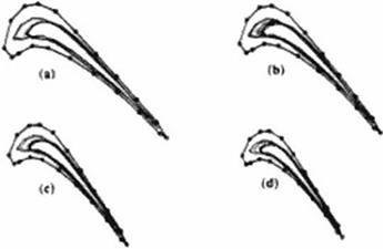
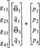
Inverse determination of unknown steady thermal boundary conditions when temperature and heat flux data arc not available on certain boundaries is an ill-posed problem [256)-(264) (Figure 85). In this case, additional overspecified measurement data involving both temperature and heat flux are required on some other, more accessible boundaries or at a finite number of points within the domain. For example, when using a BF. M algorithm, if at all four vertices designated with subscripts 1,2,3. and 4 of a quadrilateral computational gnd cell the heat sources pi are known.

at two vertices both temperature 0 as 0 and heat flux q = q arc known, while at the re-

maining two vertices neither Q or q is known, the boundary integral equation becomes

(88)

Here, coefficients of (h) and |g) matrices arc all known because they depend on gcomet nc relations and the configuration is known. In order to solve this set. all of the unknowns will be collected on the right-hand side, while all of the knowns are assembled on the left. A simple algebraic manipulation yields the following set:

— m

*11 ~#,2 *13 ”#i4

*21 ”#22 *23 ”#24 » •

*31 “#32 *33 ”#34 *41 “#42 *43 -#44

Since (he entire right-hand side is known, it may he reformulated as a vector of known*. {¥). The left-hand side remains in the form [A){X}. Also, additional equations may be added to the equation set if. for example, temperature or heat flux measurements are known at certain locations within the domain. In general, the geometric coefficient matrix [Л] will be non-square and highly ill-conditioned. Most matrix solvers will not work well enough to pro­duce a correct solution. There exists a very powerful technique for dealing with sets of equa­tions that are either singular or very close to singular These techniques, known as Singular Value Decomposition (SVD) methods |265], arc widely used in solving most linear least squares problems. Thus, using an SVD algorithm it is possible to solve for the unknown surface temperatures and heat fluxes very accurately and non-iteratiscly. If the general formulation of the problem is to be done with finite elements or any other numerical technique instead of BEM, the inverse boundary condition determination problem would become iterative and would require special regularization methods to keep it stable.