Our heavyweight helicopter equal in the world does not have
In Rostov started production of the most load-lifting rotary-wing car The Russian holding «Helicopt[...]

Everything about aircrafts and helicopters. News and events in aviation worldwide. Civil, transportation, military helicopters and airplanes.

Everything about aircrafts and helicopters. News and events in aviation worldwide. Civil, transportation, military helicopters and airplanes.

Everything about aircrafts and helicopters. News and events in aviation worldwide. Civil, transportation, military helicopters and airplanes.

Everything about aircrafts and helicopters. News and events in aviation worldwide. Civil, transportation, military helicopters and airplanes.


During the past dozen years, the author’s research team has been developing a unique inverse shape design methodology and accompanying software which allows a thermal system designer to determine the minimum number and correct sizes, shapes, and locations of coolant passages in arbitrarily-shaped internally-cooled configurations |238]-(255| The designer needs to specify
boih the desired temperatures and heat fluxes on the hot surface, and either temperatures or convective heat coefficients on the guessed coolant passage walls. The designer must also provide an initial guess of the total number, sizes, shapes, and locations of the coolant flow passages. Afterwards. the design process uses a constrained optimization algorithm to minimize the difference between the specified and computed hot surface heat fluxes by automatically relocating, resizing, reshaping and reoncnting the initially-guessed coolant passages. All unnecessary’ coolant flow passages arc automatically reduced to a very small size and eliminated while honoring the specified minimum distances between the neighboring passages and between any passage and the thermal barrier coating if such exists.
This type of computer code is highly economical, reliable and geometrically flexible if it utilizes the boundary element method (BBM) instead of finite clement or finite difference method for the thermal field analysis. The В EM docs not require generation of the interior grid and it is non-itcrativc (238). (239). Thus the method is computationally efficient and robust. The resulting shapes of coolant passages arc smooth,- and easily manufacturable.
The methodology has been successfully demonstrated on 2-D coated and non-coatcd turbine blade airfoils (240)-{249). scramjet combustor struts (252). and 3-D coolant passages in the walls of 3-D rocket engine combustion chambers (253) and 3-D turbine blades (254). [2551.
Nonlinear BEM algorithms are the best choice for the thermal analysis because of their computational speed, reliability (due to their non-iterative nature) and accuracy with elliptic type problems. A simple method for escaping local minima has been implemented and involves switching the objective function when a stationary point is achieved |245). An accurate method, based on cxponcntal spline fitting and interpolation of the cost function values, has been developed for finding the value of optimal search step parameter during gradient search optimization (244). It is also possible to develop a version of the 3-D inverse shape design code that will allow for multiple realistically shaped coolant flow passages with an arbitrary – number of fins or ribs in each of the passages (252) and prespecified locations of struts (242). In addition, this version of the 3-D inverse design code could allow for a variable thickness, segmented and non – segmented thermal barrier coatings with temperature-dependent thermal conductivities.
G. S. Dulikravich
The Pennsylvania Stale University, University Park, PA. USA
13.1 Introduction
During the design of high speed flight vehicles the designer should take into account the aerodynamic heating due to surface friction and the high temperature air behind the strong shock, waves The allowable exterior surface temperatures arc limited by the material properties of the skin materia) of the flight vehicle. In addition, the amount of heat that penetrates the skin structure should be minimized since it will have to be absorbed by the fuel and not allowed to enter the passenger cabin. A typical remedy is to cool the structure by pumping a cooling fluid (typically the fuel) through numerous passages manufactured inside the outer structure of the flight vehicle. A design optimization method should therefore provide the designer with a tool to guide the development of innovative designs of internally cooled, thermally coated or non-coated structures that will cost less to manufacture, have a longer life span, be easier to repair, and sustain higher surface temperatures
With the increasing number of variables that need to be optimized, the discrete function space containing the optimization variables tends towards a continuous function space for which it is possible to use a global analytical formulation tan adjoint system) instead of the local discretized formulation (gradient search and genetic evolution algorithms). The control theory (adjoint operator) concept is essentially a gradient search optimization approach where the gradient information is obtained by formulating and solving a set of adjoint partial differential equations rather than evaluating the derivatives using finite differencing Like the classical optimization algorithms, the control theory (adjoint operator) formulation can be used either for optimizing a 3-D aerodynamic shape by maximizing its lift, minimizing drag. etc., or it can be used as a tool to enforce the desired surface pressure distribution in an inverse shape design process. If the governing system of partial differential equations is large and the solution space is relatively smooth, then the control theory (adjoint operator) approach is more appropriate than the classical optimization approaches (216J-|2I8). The mathematical formulation is very involved and was only briefly sketched in the previous lecture.
There have been several approaches at creating an aerodynamics control theory (adjoint operator) formulation [216)-I233|. The early efforts (2I6]-[220| were highly mathematical. hard to understand and computationally intensive. Since then, two similar approaches have been followed by most researchers. They are associated with the research teams of Professor A. Jameson (22lJ-[225) who adopted and extended the previous effons by the French researchers, and the research team of Professor V. Modi I226j-(228j who followed a more comprehensible mechanistic approach practised by researchers in the general fields of inverse shape design in elasticity and heal conduction.
To date, successful and impressive results have been obtained by both research groups where Jameson’s group focused on transonic mviscid flow model and Modi’s group focused on incompressible viscous laminar and turbulent flow models of the flow field Published results of 3-D elbow diffuser and airfoil shape optimization using the adjoint operator approach and incompressible laminar and turbulent flow Navicr-Stokes equations (226)-|228) suggest that a typical optimized design consumes the amount of computing time that is equivalent to between 20 • 40 flow-held analysis (Figure 81. Figure 82). Similar total effort (an equivalent of 30 * 60 flow-field analysis) was reported for 3-D transonic isolated wing design using Euler equations |2I. 22). Tills could be compared with several hundreds and even thousands of flow analysis runs when using a typical genetic algorithm or a typical gradient search optimization algorithm. These results dispel earlier reservations (30) that adjoint operator approach formulations might not be computationally cflicicnt since they involve the solution of the governing flow-field equations. an additional set of adjoint equations, and several more interface partial differential equations.
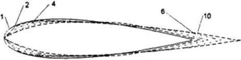
 History of the iterative evolution of a minimum drag airfoil starting from a NACA0018 airfoil at Re = 5000. Labeling numbers correspond to the iterative cycles each consisting of one flow-field analysis and one solution of the adjoint system [228].
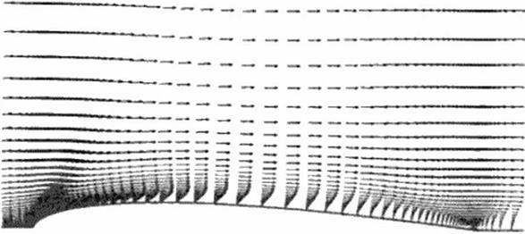
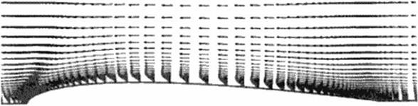
Although very impressive and mathematically involved, the general control theory (adjoint operator) approach has certain problems. One drawback is that it does not always allow for flow separation. The method also suffers from tendency to converge to any of the numerous local minima like most of the gradient search optimizers. An additional drawback is that it requires the derivation of an entirely new system of partial differential equations in terms of some non-physical adjoint variables and specification of their boundary conditions. Choosing correct boundary conditions for the adjoint system is quite a challenge since the adjoint variables are not physical flow quantities 1228]. There arc many ways to derive the adjoint system and some additional partial differential equations coupling the onginal system and the adjoint system (221)-[226). If the adjoint system of partial differential equations is different from the original system of the flow-field governing equations, a significant effort needs to be invested in separately coding the two systems. If the adjoint system is almost the same as the original governing system, the numerical algorithms for the two systems arc practically the same and the entire approach could be implemented more readily using the existing CFD analysis software (228J. Actually, if the adjoint system has the same form as the flow-field governing system except that the sign of the convective term in the adjoint system is negative, the solution of the adjoint system will represent a flow in the reverse direction (Figure 83 and Figure 84).
The complexity of the enure adjoint operator formulation makes it difficult to comprehend. implement and modify. Moreover, the adjoint operator formulation is very specific and different formulation needs to be developed and coded for each flow field model (Euler, parabolized Navier-Stokcs. Navier-Stokes. etc.) The control theory (adjoint operator) approach is very attractive if the designers want to use only one specific flow-ticld analysis axle as the basis for a design code and if they want to perform design in only one discipline (for example, aerodynamic shape design only). Since the designers use a variety of progressively more sophisticated design codes during the design process and since the design objectives are inherently multidisciplinary, the control theory (adjoint operator) approach can hardly be justified in the context of the multidisciplinary objectives, funds typically available, and the time limits imposed on the designer
In die case of a truly multidisciplinary problem, a new adjoint sy stem would have to be derived and coded to solve several adjoint systems simultaneously. Since each disciplinary analysis and adjoint system usually has vastly different time scales, the combined multidisciplinary analysis and adjoint system would have a slow convergence rale and an overall marginal stability because of a very large number of local minimums. Reliability of such a design system might be questionable since it is known that sensitivity derivatives for highly non-linear systems might be discontinuous [207J The adjoint system must be discretized for an apptoximation to the gradient to be found. This approach is less reliable than the implicit function theorem approach (231), (2321. Therefore, finding the gradients of the objective function using information from the discretized flow-field governing equations is more reliable (2321 than if an analytic expression for the gradient is derived in terms of the exact flow-field solution and the solution to the adjoint sy stem [223].
|
Figure 83 Horizontal components of the fluid velocity vector at different axial locations; the flow is from left to right [228]. |
|
Figure 84 Horizontal components of an adjoint variable at different axial locations; the "flow" of the adjoint vector is in the opposite direction to the physical fluid flow if the adjoint system is made to resemble the flow-fleld governing system except for the change in sign of the convective term [228]. |
An attractive extension of the control theory (adjoint <*perator) approach represents the "one-shot" method [234M237J. It implicitly combines a multigrid solution technique with the classical control theory for systems of partial differential equations. Consequently, this approach is faster than the regular control theory (adjoint operator) approach where the multi – grid technique was used only to accelerate the flow-field analysis code 1225). Nevertheless, the "one-shot”’ formulation and implementation are even more complex than the control theory (adjoint operator) formulation, and it suffers from similar reliability issues due to the fact that it might be equally prone to the local minima
12.3 Conclusions
A number of existing and emerging concepts and methodologies applicable to automatic inverse design and optimization of arbitrary realistic 3-D configurations have recently been surveyed and compared [2351. These attempt* to classify the design methods and to expose their major advantages and disadvantages resulted in the following conclusions:
• control theory (adjoint operator) algorithms offer very economical shape design optimization although they arc complex to understand and develop, hard to modify, too field-specific. and prone to local minima.
• one-shot method should be further researched as an esen more economical possible successor to the adjoint operator formulations w ith all of its drawbacks, and
• combination of hybrid genetic/gradient search constrained optimization of surface pressure distribution followed by transpiration inverse design offers an attractive approach in the immediate future because of its unsurpassed robustness and acceptable computing cost.
G. S. Dulikravich
The Pennsylvania State University, University Park, PA, USA
12.1 Introduction
The main drawback of using constrained optimization in 3-D aerodynamic shape design is that it requires anywhere from hundreds to tens of thousands of calls to a 3-D flow-field analysis code. Since certain general 3-D aerodynamic shape inverse design methodologies require only a few calls to a modified 3-D flow-field analysis code, it would be highly desirable to create a hybrid new design algorithm that would combine some of the best features of both approaches while requiring less computing time than a few dozen calls to the 3-D flow-field analysis code. We will discuss two such hybrid design formulations that have been proven to work and are distinctly different from each other.
12.2 Target Pressure Optimization Followed by an
Inverse Design
The unique feature of this concept (204). (205) is that it offers the most economical approach to constrained aerodynamic shape optimization. It consists of two steps: surface pressure constrained optimization follow ed by an inverse shape design. This approach avoids most of the limitations of the inverse shape design while requinng considerably less computing time than the direct geometry optimization.
 |
Surface pressure optimization phase of this design approach starts by parameterizing the initial surface pressure distribution using (3-splines (206). Typically, between five and ten control points in the ^-spline representation are sufficient to describe the pressure distribution on the upper surface and the similarly small number of control points is sufficient for representation of the pressure distribution on the lower surface of a two-dimensional (2-D) section of the 3-D object. For example, if 7 control points are used to parameterize the upper surface pressure distribution and 7 control points are used to parameterize the lower surface pressure distribution (Figure 78). then 4 control points will have to be used to fix the locations of leading and trailing edge stagnation points. Constraints can be introduced at this stage by specifying the slopes of the pressure distribution at the leading edge. This will require fixing one additional control point on the upper and the lower surface pressure distribution (204]. The steeper the leading edge pressure distribution variation, the larger the leading edge radius of the resulting 2-D aerodynamic section will be. The optimization of the constrained surface pressure distribution can then be achieved (207]. (208] by optimizing the 8 "floating” control points each defined by its x – coordinatc and the corresponding value of pressure. The optimization is thus performed on surface pressure distribution, not on the actual aerodynamic shape.
This means that the perturbations introduced in the surface pressure distribution during the optimization will have to be somehow related to the global objectives like aerodynamic lift, drag. etc. These global aerodynamic parameters depend on the geometric shape of the object and on the pressure distribution on its surface. It is therefore necessary to relate the geometry of the object and the surface pressure distribution. This is precisely what a typical flow-field analysis code should do except for the fact that geometry of the object is not known yet. A possibility would be to run an inverse shape design code for each surface pressure perturbation and then to integrate the surface pressure in order to evaluate the corresponding lift. drag. etc. This is
obviously an unacceptably, inefficient approach.
Instead, the guessed surface pressure distribution can be optimized without ever calling a flow-field analysis code or the inverse shape design code. To accomplish this, use is made of extremely efficient approximate relations 1209). |2I0| relating the integrated surface pressure distnbution and the object s maximum relative thickness (209), specified location of the flow transition points, and the aerodynamic drag with any of the classical boundary layer solutions (210). Then, the optimization of the few coefficients, for example, of {3-spline parameterization of the surface pressure distnbution curves on each 2 D section can be performed reliably and economically using an optimization algorithm [211], (204). (212). Optimization of the surface pressure distnbution parameters, instead of directly optimizing the 3-D geometry parameters, has several advantages: the total number of optimization variables is reduced, the range of (3- splinc coefficient variations can be large, the design space docs not have an excessive number of local minima, and the sensitivity derivatives do not have discontinuities This procedure easily accepts constraints on surface pressure distribution such as the desired slopes of the curves at the leading and trailing edges, the maximum value of negative coefficient of pressure, a condition that the surface pressure distribution curves on the upper and the lower surface never cross each other thus avoiding locally negative lift force. These optimization tasks can be reliably achieved using a genetic evolution optimization algorithm (204). although an even more reliable and computationally faster approach would be to use a hybrid genetic/gradient search optimization algorithm (212). (213).
The second phase of this combined 3-D shape design procedure utilizes the optimized surface pressure distribution and any of the fast inverse shape design algorithms (214). (204), (215) to find the corresponding 3-D configuration (Figure 79).
The entire two-step design algorithm requires a minimum development lime since (3- spline discretization codes, constrained optimization codes, flow-field analysis codes, and inverse design codes are available to most aerodynamicists. If the optimized surface pressure distribution results in a 3-D geometry which violates some of the local geometric constraints, the computed pressure at the constrained points can be used instead of the optimized local pressure Moreover, this approach gives the designer a partial control of the key elements of the design by asking him to specify a few key bounding features of the "good" surface pressure distribution and then lolling the robust and fast optimizer find (he details of the optimal pressure distribution. Using this approach to shape optimization the designer also has the ability to visually control and terminate or restart the design process if he decides that the values of some of his specified constraints could be improved.
The method offers the most economical and robust approach to 3-D constrained aerodynamic shape optimization (Figure 80> that consumes approximately 5 – 10 times the computing time needed by a single 3-D flow-field analysis (204). This is much more cost-effective than (ho classical approach of simultaneously optimizing the surface pressure distribution and the corresponding 3-D geometry w hich costs an equivalent of hundreds and even thousands of flow field analy sis runs.
Modified geometry and preuure distribution. F(ntl dittnbution» (*>
(*) after five ucra&oni after not iteration}
Figure 80 An example of a convergence history of target pressure optimization followed by transpiration inverse design [204].
The GA has proven itself to be an effective and robust optimization tool for large variable-set problems if the cost function evaluations arc very cheap to perform. Nevertheless, in the field of 3-D aerodynamic shape optimization we arc faced with the more difficult situation where each cost function evaluation is extremely costly and the number of the design variables is relatively large. Standard GA will require large memory if large number of design variables arc used. The number of cost function evaluations per design iteration of a GA increases only mildly with the number of design variables, while increasing rapidly w ith the increased size of the initial population. Also, the classical GA can handle constraints on the design variables, but it is not inherently capable of handling constraint functions (198). Thus, the brute force application of the standard GA to 3-D aerodynamic shape design optimization is economically unjustifiable.
Consequently, a hybrid optimization made of a combination of the GA and a gradient search optimization or the GA and an inverse design method has been shown be an advisable way to proceed (180]. (20l]-(203). Preliminary results obtained with different versions of a hybrid optimizer that uses a GA for the overall logic, a quasi-Newtonian gradient-search algorithm or a feasible directions method [167) to ensure monotonic cost function reduction, and a Nelder-Mead sequential simplex algorithm or a steepest descent methodology of the design variables into feasible regions from infeasible ones has proven to be effective at avoiding local minima Since the classical GA docs not ensure monotonic decrease in the cost function, the hybrid optimizer could store information gathered by the genetic searching and use it to determine the sensitivity derivatives of the cost function and all constraint functions (203). (180). When enough information has been gathered and the sensitivity derivatives arc known, the optimizer switches to live feasible directions method (with quadratic subproblem) for quickly proceeding to further improve on the best design.
One possible scenario for a hybrid genetic algorithm can be summarized as follows:
• Let the set of population members define a simplex like that used in the Ncldcr-Mcad method.
• If the fitness evaluations for all of the population members docs not yield a better solution, then define a search direction as described by the Nelder-Mead method.
• If there arc active inequality constraints, compute their gradients and determine a new search direction by solving the quadratic subproblcm.
• If there are active equality constraints, project this search direction onto the subspace tangent to the constraints
• Perform line search.
Our recent work [203]. |180) indicates that the hybrid GA can yield answers (Figure 75 and Figure 76) not obtainable by standard gradient methods at comparable convergence rates (Figure 77). This hybrid optimizer can also handle non-lincar constraint functions, although the main computational cost will be incurred by enforcing the constraints since this task will involve evaluating the gradients of the constraint functions.
|
|
|
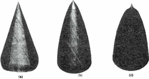
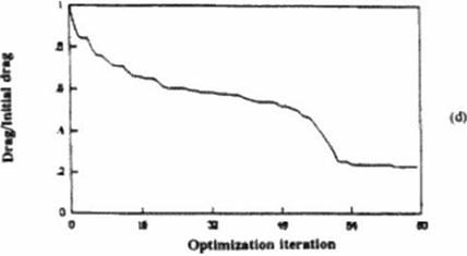
Figure 75 Our hybrid gradient search/genetk constrained optimizer keeps on improving the design even beyond the known analytic optimal solution (von Karman and Sears-Haack smooth ogives). It transformed an initially conical configuration (a) with 100% drag into a smooth ogive shape (b) with 56% drag and finally into a star-shaped spiked missile (c) with only 22% of the initial drag. Convergence history (d) shows monotonic convergence although 480 variables were optimized with a constrained volume and length of the missile [203], (180). |
![]()
 |
||
Starting from an initially conical body at zero angle of attack and a hypersonic oncoming flow, the hybrid G. Vgradient search constrained algorithm arrived at this smooth, cambered 3*1) lifting body with a maximized value of lift-to-drag while maintaining the initial volume and length [2031,(180].
![]() Comparison of convergence histories of a constrained gradient search and a constrained hybrid genetic/gradient search optimizer for example shown in Figure 76, [203], 1180].
Comparison of convergence histories of a constrained gradient search and a constrained hybrid genetic/gradient search optimizer for example shown in Figure 76, [203], 1180].
11.5 Conclusions
From the brief survey of positive and negative features of different optimization algorithms it can be concluded that:
• brute force application of gradient search sensitivity-based optimization methods is very computationally intensive and unreliable for large aerodynamic problems since they are prone to local minima.
• brute force application of genetic evolution optimizers is very computationally intensive for realistic 3-D problems that involve a number of constraints, and
• use of hybrid gcnetic/gradient search coastrained optimization algorithms offers the most reliable performance and the best convergence.
Besides a wide variety of ihc gradient-based optimization algorithms, truly remarkable results were obtained using an evolution type generic algorithm or GA 1168).(169).| 191J. The GA methods simulate the mechanics of natural genetics for artificial systems based on operations which arc the counter parts of the natural ones. They rely on the use of a random selection process which is guided by probabilistic decisions. In genera!, a GA is broken into three major steps: reproduction. crossover, and mutation An initial population of complete design variable sets are analyzed
according to some cost function. Then, this population is merged using a crossover methodology to create a new population. This process continues until a global minimum is found. Generally, the design variable set that corresponds to the minimum point of the cost function will be representative as having the most "succcssfur features of previous "generations" of designs in the optimization process.
Although the standard genetic algorithm (GA) is computationally quite expensive since it requires a large number of calls to the flow-field analysis code, the robustness of this algorithm and the case of its implementation have created a recently renewed interest in applying it for aerodynamic shape design (192)-(201). Nevertheless, the examples presented in these publications involve aerodynamic shape optimization with a small number of design variables that form a relatively compact function space. Solutions of such optimization problems would be considerably more efficient when using more common gradient search algorithms Moreover, none of the examples in these publications attempt to treat equality-type constrained optimization which represents the most difficult problem for a typical GA algorithm. The classical GA can handle constraints on the design variables, but it is not inherently capable of handling constraint functions (198) Most of the recent publications involving the GA and aerodynamic shape optimization have involved problems posed in such a way as to eliminate constraint functions. or to penalize the cost function when a constraint is violated. These treatments of constraints reduce the chance of arriving at the global minimum.
Probably the most attractive feature of the GA is its remarkable robustness since it is not a gradient-based search method The GA is exceptional at avoiding local minima, because it tests possible designs over a large design variable space Hence, the GA is especially suitable for handling a large number of design variables that belong to widely different engineering disciplines. thus making it particularly suitable for true ompkx multidisciplinary coptimization problems. Tire GA is especially suitable for the types of problems where the sensitivity derivatives might be discontinuous (I73J which is sometimes the problem in 3-D aerodynamic optimization The number of cost function evaluations per design iteration of a GA docs not depend on the number of design variables. Rather, it depends on the size of the initial population.
There are some subtleties associated with tlie GA that, if treated properly, greatly increases the effectiveness and usefulness of the method. One such subtlety involves the crossover procedure When two members of the population arc chosen for a crossover, their design variable sets arc generally encoded into strings called "chromosomes *. After a crossover has taken place, the "child" variable set is recovered by decoding its newly created chromosome string. When the design variables are floating-point numbers, as is usually the case, this coding and decoding process can introduce a loss of precision arising from numerical truncation on a finite precision computer. This is particularly true when the chromosome string format is defined by a "bit-string" (a base 2 number», and the operating language is FORTRAN A crossover method that preserves full precision in the design variables can be developed (202J by changing the format of the coded chromosome string and by the implementation of C and C++ as the operating language instead of FORTRAN. These languages allow bitwise shifting of floating point numerics and require no coding or decoding processes whatsoever The C++ language further allows object-oriented programming techniques that provide a platform for the truest genetic interaction of design variable sets. Equality and non-equality constraints can be incorporated by using RoSen’s projection method (202J.| 180). This improved GA could be used as a black box optimizer in aerodynamics, elasticity, heal transfer, etc, or in a multidisciplinary design optimization.
It is often desirable to have a capability to predict the behavior of the inputs to an arbitrary system by relating the outputs to the inputs via j sensitivity derivative matrix [ !84]-( 188). while treating the system as a black box. The sensitivity derivative matrix can be used for the purpose of controlling the system outputs or to achieve an optimized constrained design that depends on the system outputs The objective is to generate approximations of the infinite dimensional sensitivities and to transfer these approximate derivatives to the optimizer together with the approxmiatc function evaluations. The control vanables are then updated with the sensitivity derivatives which are the gradients of the cost function with respect to the control variables. The general concepts for the sensitivity analysis can be summarized as follows (185)
The system of governing flow-field governing equations after discretization results in a system of non-linear algebraic equations
where Q is the vector of the solution variables in the flow-field governing system. X is the computational gnd and D is the vector of design variables (for example, coordinates of 3-D aerodynamic shape surface points). Hence
![]()
![]() dR _ dRdQ dRdX Э R dD ^QdD + dXdD + dD
dR _ dRdQ dRdX Э R dD ^QdD + dXdD + dD
Similarly, aerodynamic output functions (lift. drag. Iift/drag. moment, etc.) are defined as
F = F(Q(D),X{D),D)
Hence
dF _ dFdQ. dFdX. dF dD = bQdD * bXdD + ДО
System (81) is solved for the sensitivity derivatives of the field variables, dQ/dD, which arc then substituted into the system (83) in order to obtain the sensitivity derivatives of the desired aerodynamic outputs. dF/dD. This approach is typically used if the dimension of F is greater than that of D which is seldom the case in a 3-D aerodynamic shape design.
When die number of design variables D is larger than the number of the aerodynamic output functions F. it is more economical to avoid solving for dQ/dD This can be accomplished by using an adjoint operator approach where a linear system
)’-&)’-»
must be solved first. Here. A is a discrete adjoint variable matrix associated with the aerodynamic output functions. F. Substituting equation (84) into equation (83). it follows from equation (81) that the aerodynamic output derivatives of interest can be computed from
dF _ AT (dRdX dR dFdX dF
dD ~ A ЛЯШ + ШЇГШо + ‘Зо (85)
This quasi-analytical approach to computing sensitivity derivatives is more economical and accurate than when evaluating the derivatives using finite differencing. Nevertheless, sensitivity analysis is a very costly process requiring a large number of analysis runs.
In the gradient-search optimisation approach the flow analysis cixlc must be called at least once for each design variable in order to compute the gradient of the objective function
during each optimization cycle. Since each call to the analysis code is very expensive, such an approach to design is justified only if a small number of design variables is used. In the ease of a 3-D design, this is hardly justifiable even if one uses 3-D surface geometry paramctnzation which severely constrains 3-D optimal configurations.
One of the most promising recent developments in the aerodynamic shape design optimization is a method that treats the entire system of partial differential equations governing the flow-field as constraints, while treating coordinates of all surface gnd points as design variables (189). This approach eliminates the need for geometry parameterization using shape functions to define changes in the geometry. Since fluid dynamic variables. Q. are treated here as the design variables, this method allows for rapid compulation of partial derivatives of the objective function with respect to the design variables. This approach is straightforward to comprehend and efficient to implement in Newton-type direct flow analysis algorithms where solutions of the equations for dQ/dD or A amount to a simple back-substitution The problem is that the classical Newton iteration algorithm is practically impossible to implement for 3-D aerodynamic analysis codes because of its excessive memory requirements when performing direct LU factorization of the coefficient matrix.
 |
|
Instead of using an exact New ton algorithm in the flow-analysis code, it is more cost effective to use a quasi-Newton iterative formulation or an incremental iterative. strategy (I85j. [ 190) given in the form
![]() could be any fully-converged numerical approximation of the exact Jaco
could be any fully-converged numerical approximation of the exact Jaco
bian matrix.
G. S. Dulikravich
The Pennsylvania Stale University, University Park, PA. USA
11.1 Introduction
Although fast and accurate in creating aerodynamic shapes compatible with the specified surface pressure distribution, the inverse shape design methods create configurations that arc not optimal even at the design operating conditions [ 163). 1164] At off design conditions, these configurations often perform quite poorly except w hen the specified surface pressure distribution, if available at ail. would be provided by an extremely accomplished acrodynamicist. When using inverse shape design methods, it is physically unrealistic to generate a 3-D aerodynamic configuration that simultaneously satisfies the specified surface distribution of flow variables, manufacturing constraints (smooth variation of a lifting surface sweep and twist angles, smooth variation of its taper, etc.) and achieves the best global aerodynamic performance (overall total pressure loss minimized. Iifl/drag maximized, etc ). The designer should use an adequate global optimization algorithm that can utilize any available flow-field analysis code without changes and efficiently optimize the overall aerodynamic characteristics of the 3-D flight vehicle subject to the finite set of desired constraints. The constraints could be purely geometrical or they can be of the overall aerodynamic nature (minimize overall drag for the given values of flight speed, angle of attack and overall lift force, etc ). These objectives can only be met by performing an aerodynamic shape constrained optimization instead of an inverse shape design.
The size and shape of the mathematical space that contains all the design variables (for example, coordinates of all surface points) is very large and complex in a typical 3-D case. To find a global minimum of such a space requires a sophisticated numerical optimization algorithm that avoids local minima, honors the specified constraints and stays within the feasible design domain The design variable space in a typical aerodynamic shape optimization has a
number of local minima. These minima are very hard to escape from even by switching the objective function formulation [165) or consecutive spline fitting and interpolation of the unidirectional search step parameter (166).
There are several fundamental concepts in creating an optimization algorithm. One family of optimisation algorithms is based on reducing the objective or cost function (for example. aerodynamic drag) by evaluating die gradient of the cost function and then updating the design variables in the negative gradient direction (167). Evolution search or genetic algorithms is another family of optimization algorithms that is based on a semi-random sampling through the design variable space and docs not require any gradient evaluations [168). |I69|. Since both families of optimization algorithms require flow-field analysis to be performed on every perturbed aerodynamic configuration, the optimization of 3-D aerodynamic shapes is a very computationally intensive task
In a gradient-search optimization approach the flow analysis code must be called at least once for each design variable during each optimization cycle in order to compute the gradient of the objective function if one-sided finite differencing is used for the gradient evaluation. If a more appropriate central differencing is used for the gradient evaluation, the number of calls to the 3-D flow-field analysis code will immediately double Despite this, the optimization algorithms arc still often misused to minimize the difference between the specified and the computed surface flow data in inverse shape design – a task that is significantly more economical when accomplished w ith any of the standard inverse shape design algorithms.
 |
The most serious drawback of the brute force application of the gradient search optimization in 3-D aerodynamics is that the computing costs increase nonlincarly with the growing number of design variables thus making these algorithms suitable for smaller optimization problems. On the other hand, the computing cost of using evolution search algorithms increases only moderately with the number of design variables (Figure 74) thus making these algorithms more suitable for large optimization problems. Only these optimization algorithms that require minimum number of calls to the flow-field analysis code will be realistic candidates for the 3-D aerodynamic shape optimization
Since the actual 3-D flow-field analysis codes of Euler of Navicr-Stokes type arc very lime consuming, the designer is forced to restrict the design space by working with a relatively small number of the design variables for parameterization (fitting polynomials» of either the 3-D surface geometry (17()|-(172J or the 3-D surface pressure held 1173]. [174]. The optimization code then needs to identify the coefficients in these polynomials. The most plausible choices arc cubic splines. Chebyshev and Fourier polynomials [I75]-(177] are not advisable because they become excessively oscillatory with the increasing number of terms in the polynomial. Moreover, when perturbing any of the coefficients in such a polynomial, the entire 3-D shape will change. Since it is absolutely necessary to constrain and sometimes disallow motion of particular parts of the 3-D surf ace, the most promising choices for the 3-D parameterization appear to be different types of b-splincs 1178], (179), 1171 ]. (180]. local analytical surface patches
[181] . and local polynomial basis functions 1182]. Only when it is possible to use simple and very fast flow-field analysis codes could we afford an ideal optimization situation where each surface grid point on the 3-D optimized configuration is allowed to move independently.
Single-cycle optimization (183] oilers one viable approach at reducing the computing costs. Here, the flow-field analysis code is run on each perturbed aerodynamic configuration for only a small number of iterations (instead to n full convergence» before an optimizer is used to determine the new geometry. An optimal aerodynamic shape is then found by optimally weighing each of the number of feasible configurations that can be obtained using inverse design methods. Hence, this optimization approach guarantees that the final configuration will he realistically shaped and manufacturable, although the range of geometric parameters to be optimized is limited by the geometry’ of the extreme members of the original family of configurations.
|
.2 .2 Л -ДДО ♦ – Ддо ♦ -^-ДО дх2 Эу2 Э* |
|
3х+Тх* |
An attractive property of integral equations is that the influence of the boundary conditions is transmitted throughout the flow – field instantaneously in the case of a linear flow problem. Even for non-linear flow problems the influence of the boundary conditions is transmitted throughout the flow-field extremely quickly as compared to the partial differential equation models where the finite difference or finite element discretization allows the influence of the boundary conditions to be transmitted at most one grid cell per dunng each iteration. Л very fast and versatile 3-D aerodynamic shape inverse design algonthm was developed and is w idely utilized in several countries I I58J-[ 161]. It can accept any available 3-D flow-field analysis code as a large subroutine to analyze the flow around the intermediate 3-D configurations. The configurations arc updated using a fast intcgro-diffcrential formulation where a velocity potential perturbation OU. y./) around an initial 3-D configuration zw.(x. y) can be obtained from, for example, a Navi – er-Stokes code [ 1611. Here, the subscripts ♦/- refer to the upper and lower surfaces of the flight vehicle. Transonic 3-D small perturbation equation is
Here, differentially small potential perturbation is Atyx. y.z) and x. y.z coordinates have been sealed via Prandtl-Glaucrt transformation, V^, is the free stream magnitude, while
(77)
Here. M is the local Mach number and a^, is the free stream speed of sound. The floss tangency condition is then
![]() iU*Uy.*M» = Vm |^wU. y)
iU*Uy.*M» = Vm |^wU. y)
Since —Дф(лг, у, ♦/■О) can be obtained from equation (75). the 3-D geometry is
dZ
readily updated from
bz^ (x, y) ш Jj-(Ae+(x. jr)^ Az (jr, y)l</jf± | J^{Ae4,(jr. y)-Ae,(Jby)I</» (79)
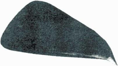
![Подпись: Figure 73 Winglets on a Japanese space plane were successfully redesigned using the integro-differential equation approach and a Navier-Stokes flow-field analysis code [161].](/img/3131/image154_3.gif) |
Since equation (75) is linear, it can be reformulated using Green’s theorem as an intc – gro-dilTcrential equation. The Г term on the right hand side of equation (75) would require volume integration which can be avoided if Г is prescribed as smoothly decreasing away from the 3-D flight vehicle surface where it is known. Then, the problem can be very efficiently solved using the 3-D boundary clement method This inverse shape design concept has been successfully applied to a vancly of planar wings [ 158J-[ 160] and wing-body configurations including the H-II Orbiting Plane with wingleis (161), f 162] where 3-D flow-field analysis codes were of the full potential. Euler and Navier-Stokes type. The method typically requires 10-30 flow analysis runs with an arbitrary flow solver and as many solutions of the linearized inlcgro-diffcrcn – tial equation.
10.2 Conclusions
Several prominent and proven methods that arc applicable to inverse design of 3-D aerodynamic shapes have been briefly surveyed. The design computer codes based on these methods can be readily developed by modifying solid boundary condition subroutines in most of the existing flow-field analysis codes. Thus, all of the design methods surv ey ed are computationally economical since they require typically only a few dozen calls to the 3-D flow – field analysis code. Although the inverse shape design methods generate only point-designs, it was pointed out that at least two of the methods arc conceptually capable of inverse shape design for unsteady flow conditions.
The correct number and types of boundary conditions for a system of partial differential equations can be determined by analyzing eigenvalues and the corresponding eigenvectors of the system in each coordinate direction separately This approach to boundary condition treatment is called characteristic boundary conditions {155]-( 157) since it suggests one-dimensional application of certain Ricmann invariants at ihc boundaries that can be either solid or open boundaries. For example, in a 3-D duct flow, if the flow is locally subsonic at the exit, wc will be able to compute all How variables at the exit based on the information from the interior points except for one variable that we will have to specify at the exit. If the same characteristic boundary condition procedure is applied in the direction normal to the solid wall and if the desired pressure distribution is specified on die wall, this method of iteratively enforcing the boundary conditions at the wall will result in non-zero normal velocities at the wall which can he used to update the wall shape. The general concept follows.
The F. ulcr equations for 3-D compressible unsteady flows expressed in non-conscrva – tivc form and cast in a boundary-conforming, non-orthogonal. curvilinear <£,r).£) coordinate system can be transformed into
о (73)
w here Q = ф p u v w) is the transposed vector of the non-conservative primitive variables. Figcnvalucs of В are
V * °’ J(n2 * V * n;2 ) V’ V’ V’ V*a * П v* + n:2) (74)
where V ■ n ♦ Л • и ♦ n + and the local speed of sound is defined as a —
1 x У *
(Y P / P),/:: If the П-gnd lines arc emanating from the 3-D aerodynamic configuration, we can
have several situations. If 0 < V < a one eigenvalue is negative requiring a
pressure boundary condition to he specified at that surface point.
Similarly, if-a < 0. four eigenvalues will be negative requiring
s 2 ”> 1/2
pressure, velocity ratio m/(m‘ ♦ »+**) . total pressure and total temperature to be speci
fied at that surface point. This method has been show n to converge quickly for transonic two – dimensional airfoil shape design when using compressible flow Euler equations (I56].(I57J. The method might be applicable to the inverse design of arbitrary 3-D configurations |155| although no such attempts have been reported yet. If the Euler code is executed in a time-accurate mode, the specified unsteady solid wall characteristic boundary conditions will provide for a time-accurate motion of the solid boundaries which is highly attractive for the design of "smart” aerodynamic configurations. This concept is not directly applicable to viscous flow codes since velocity components at the solid w all are zero.