Category Noise Sources in Turbulent Shear Flows

Basic Assumptions – Thin-Airfoil Linearized Theory

For the mathematical statement dedicated to analytical investigations, is defined as unsteady aerodynamics any lift variation on an airfoil due to a variation in the oncoming flow (speed or angle of incidence), for which the Kutta condition of no flow around the trailing edge has to be fulfilled. Such a mechanism involves the entire airfoil section. The theoretical determina-

Basic Assumptions - Thin-Airfoil Linearized Theory

tion of £(t) would be certainly a considerable task, were the exact solution sought for each practical flow field of interest, because of the variety encoun­tered in both airfoil shapes and surrounding flow conditions. But acoustic calculations benefit from the favorable effect of the logarithmic dB-scale, and often only require a consistent approximation of £(t) in most cases of interest (rotating blades, high-lift devices). For subsonic thin airfoils with small camber and angle of incidence, referred to as slightly loaded airfoils, and small velocity fluctuations, the linearized unsteady aerodynamic the­ory described below provides helpful approximate solutions. In contrast for highly cambered, thick blades, such as the ones encountered in turbine blade rows, the linearized approach is not relevant, and a numerical analysis is required.

Подпись:Подпись: PRESSURE SIDE > Подпись:Basic Assumptions - Thin-Airfoil Linearized TheoryЛпе

«•sS»***

SUCTION SIDE TE

Figure 2. General airfoil definition. a and Z are the angle of attack and the maximum camber displacement, respec­tively.

Before listing the assumptions of the linearized thin-airfoil theory, let us perform first a rapid analysis in the two-dimensional framework of Fig. 2. U0 is the mean flow velocity, at an angle of attack a with respect to the chord line. Consider the velocity fluctuation vector u = (u, w) superimposed on the mean flow and defined in absence of airfoil. u is the variation of velocity magnitude along the average flow direction and w the variation of angle of attack.

A first insight into unsteady aerodynamics is provided by perturbing the steady-state equation relating the lift force per unit span F0 to the relative velocity U0:

Подпись: dF Basic Assumptions - Thin-Airfoil Linearized Theory

where CL is the lift coefficient, function of the angle of attack a, and c the chord length (Fig. 2). Small variations of the angle of attack and of the magnitude of the velocity vector then lead to the differential

This is a quasi-steady approximation because eq.(1) is assumed to hold also for transient flow conditions. For weakly loaded airfoils it can be assumed that CL ^ 1 ; furthermore dCL/da = 2 n for a Joukowski airfoil. It is concluded that whenever the incident velocity disturbances w and u have the same order of magnitude, the component w is responsible for the major part of the unsteady loads. The assumptions are better justified for moderately cambered airfoils or lifting surfaces. Intuitively, blowing on a flat plate parallel to its surface and varying the flow speed is not expected to induce lift variations, whereas slightly changing the angle of attack produces significant ones. In contrast, variations of the flow speed Uo at constant angle of attack on a highly cambered surface are known to also generate large lift fluctuations, as suggested by the vertical efforts exerted on an umbrella in a varying wind. As a consequence, only the fluctuations of angle of attack are generally considered in linearized unsteady aerodynamic theories applied to slightly cambered airfoils. Highly cambered airfoils are not considered here; they would require numerical investigation.

Obviously the direct proportionality and the immediate response of the airfoil expressed in eq.(1) are abusive. Indeed by virtue of the Kutta con­dition, vorticity is continuously shed in the wake as a result of any inflow variation. The evacuation of the shed vorticity in the flow requires a finite time, which results in some delay of the force variation. The quasi-steady approximation is just the asymptotic form of a needed more general de­scription; it is valid for very slow variations or for large flow patterns with respect to the dimensions of a body in a flow (see Fig. 1-a again). Part of the broadband noise from low-speed fans is predicted based on similar arguments by Sharland (1964) and Fukano et al (1977).

Anyway, as shown by the pioneering work by von Karman & Sears (1938), cited by Goldstein (1976), small thickness, camber and angle of incidence only determine the steady lift, but have no significant effect on the unsteady loads. This fundamental decoupling of the unsteady aerody­namic behavior from the mean loading has very important implications. Typically it means that lift fluctuations can be determined independently of the airfoil design by just solving the problem of the response of a thin flat

plate embedded at zero incidence in a parallel mean flow carrying normal velocity disturbances. This will be called Sears’ problem in this course.

The general approach for solving Sears’ problem in two or three dimen­sions is described now. First of all, the incident disturbances are assumed frozen, which means that their decaying time is large in comparison with a characteristic traveling time along the chord length. They are rotational in essence but the additional disturbance induced by the airfoil can be de­scribed as a potential field, apart from the wake; the part of this field which propagates away from the airfoil is precisely the acoustic motion. Secondly the solution is derived in the frequency domain because the time delay pro­duced by the Kutta condition must be compared to the characteristic period of the variations of angle of attack. The procedure is as follows.

1 – The oncoming velocity disturbance normal to the airfoil surface (up – wash) is Fourier-analyzed. Each Fourier component defines a transverse sinusoidal gust in the sense of unsteady aerodynamics. A gust is charac­terized by the chord-wise aerodynamic wave number k1 and, because of the convection speed U0 , induces forces on the airfoil at the corresponding an­gular frequency ш = k1 U0 . A spanwise aerodynamic wavenumber k2 is also introduced when the theory is extended in three dimensions (Fig.5 ).

2 – At a given value of ш or ki, the Fourier coefficient E(ki) of the total unsteady lift force is determined by some unsteady aerodynamic theory in terms of the transverse fluctuation amplitude rw(k1) . In order to connect the formal result eq.(1), it is written:

E(ki) = n po Uq w cT,

where T is some aerodynamic transfer function introduced for physical con­sistency to account for the phase shift between the lift variations and the variations of angle of attack. More precisely the local distribution of fluc­tuating lift along the chord line, say £(k1,y1) where y1 is the chord-wise coordinate, may be of interest. For acoustic purposes, the integrated lift is enough if the chord length is acoustically compact, but the distributed local lift is needed if it is not.

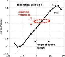
The phase shift results in an inclined hysteresis response curve in the plane (a, Cl) (Fig. 3). Instead of following the steady-state curve, the op­erating point of the airfoil follows that hysteresis loop, centered around the mean-value point. The amplitude of the lift variations is well smaller than what the quasi-steady approximation would predict. The figure also suggests that oncoming disturbances can prevent the airfoil from stall. In­deed wind-tunnel experiments and simulations on oscillating airfoils have confirmed this point.
Basic Assumptions - Thin-Airfoil Linearized Theory

Angle of attack (°)

Figure 3. Typical aerodynamic lift coefficient curve of an airfoil (steady state) and illustration of the unsteady aero­dynamic response to cyclic variations of the angle of attack.

3 – The contribution of the gust to the far-field sound is derived, based on the acoustic analogy.

In this procedure the key step is the relationship between the incident velocity disturbances, assumed known, and the associated lift variations, still to be determined. A minimum review of available theories achieving this step is given below. It must be kept in mind that in practice information about velocity disturbances is generally of easier access than information about the wall pressure on a body.

Unsteady Aerodynamics

1.3 Preliminaries

A lifting surface embedded in a disturbed flow experiences time vari­ations of both lift and drag forces. These variations are sources of sound according to the acoustic analogy. For airfoil-like designed bodies with at­tached flows considered later on, lift variations are much larger than drag forces, therefore the latter are neglected and the unsteady problem is ad­dressed based on non-viscous flow arguments. Random incident velocity disturbances cause time variations of both the magnitude and the angle of attack of the relative velocity vector experienced by the airfoil. These vari­ations induce a total instantaneous force F(t), or at a more precise level the corresponding local instantaneous lift forces distributed over the surface, noted £(t). When calculating the noise from the airfoil according to Ffowcs Williams & Hawkings’ equation, the major difficulty to deal with is the evaluation of this force field with enough accuracy. In the fluid-dynamics community, the mean value of F(t) or £(t), referred to as steady loading, is primarily addressed because only the steady-state is directly related to the aerodynamic efficiency the surface must ensure. Typically the airfoil is designed for a desired value of the mean lift coefficient CL, as a function of the angle of attack a. The fluctuations of F(t) or £(t) around the mean, essentially responsible for the noise, are much more difficult to quantify, and depend on external conditions not intrinsic to the surface design. The fluctuations bring no benefit to the aerodynamic efficiency and are only an undesirable source of noise (or vibration, even though vibrations are not addressed here). So any reduction of the unsteadiness, if possible, is a good deal from the acoustical point of view and does not essentially suffer from efficiency constraints.

Broadband Noise from Lifting Surfaces. Analytical Modeling and Experimental. Validation

Michel Roger

Ecole Centrale de Lyon

Abstract

The chapter is dedicated to the noise radiated by thin airfoils in either disturbed or homogeneous flows. This includes noise pro­duced by impingement of upstream turbulence onto a leading edge, self-noise caused by boundary-layer turbulence scattering at the trailing edge and noise due to the formation of a vortex street in the near wake. Analytical modeling is proposed in the frequency do­main, based on linearized theories of unsteady aerodynamics. The same mathematical background referred to as Schwarzschild’s tech­nique is used for all mechanisms in order that the predicted trends can be compared. In a first step the analysis is focused on the derivation of the induced lift fluctuations, acting as the sources of sound according to Ffowcs Williams & Hawkings’ analogy. The radiation properties of isolated aerodynamic wave-numbers in the sources are discussed in a second step. Next a statistical declination of the formalism is introduced, relating the source statistics to the PSD of the acoustic pressure in the far field. Finally the statistical models are assessed against experimental data.

1 Introduction

1.1 Methodology and Context

Rotating blades, wings with high-lift devices and other so-called lifting surfaces (splitter plates, spoilers…) embedded in a flow generate aerody­namic sound by various declinations of vortex dynamics. Some of them have been introduced in chapter 2. If random disturbances are carried from up­stream in the oncoming flow, they are rapidly distorted around the leading edge of the surface. This produces what is often called interaction or im­pingement noise. It is not intrinsic to the surface but rather characteristic of the incident flow, even though the surface shape may have a large influence

R. Camussi (Ed.), Noise Sources in Turbulent Shear Flows: Fundamentals and Applications, CISM International Centre for Mechanical Sciences, DOI 10.1007/978-3-7091-1458-2_5,

© CISM, Udine 2013

on the produced noise. In absence of oncoming disturbances, the surface generates its own vortex dynamics through the formation of boundary lay­ers or the onset of vortex shedding, because of the effect of viscosity. The associated acoustic signature is called self-noise because it is more intrin­sic to the incriminated surface. Most applications involve airfoil-like lifting surfaces, defined by their chord and span lengths and some cross-section de­sign. Interaction noise and self-noise include span-wise distributed sources concentrated at the leading edge or the trailing edge, and localized sources at span ends (tips of blades, flap side-edges of high-lift devices…).

In all cases the prediction of the broadband noise is made a considerable task by the random character of the flow. The corresponding mechanisms can be addressed either numerically or analytically. Typically a numerical approach, based on the recent know-how in Computational Aero-Acoustics for a direct simulation or based on hybrid techniques, can be understood as a demanding extension (more than just a special case) of Computational Fluid Dynamics. An analytical approach is conceptually different. It is dedicated to an isolated, previously identified mechanism and needs drastic simplifications and assumptions on the flow features and/or on the geome­try. The general equations are linearized and the initial problem is generally interpreted as a wave-scattering problem. This major difference makes both approaches different jobs and what can be expected from one or the other one cannot fit with the same ambitions. The numerical techniques are aimed at understanding the tiniest details of the sound generating mechanism and describing or reproducing it as accurately as possible. This is achieved at the price of heavy, time-consuming computations. Some of them are not tractable yet for the Reynolds and Mach numbers of interest, making the field still open for further progress. Conversely the analytical investigations are aimed at providing approximate but very fast and cheep results. The previously required recognition of a mechanism makes the solution clearly expressed as a function of the main parameters of the flow, thus the solution itself is easily used to get information on the scaling laws and the underlying physics. This is very useful for preliminary design in engineering context. Within the scope of hybrid approaches, an analytical prediction model can also be used to deduce the far-field sound by post-processing an already available simulation of the flow. It is clear that both approaches remain necessary in any case, and for the both of them significant improvements and new achievements are made every year in the community of aeroa – coustics. On the one hand, numerical techniques become more and more attractive and tractable. On the other hand, analytical techniques can still be extended and thus have not yet reached their limitations. The present chapter is dealing more specially with flows developing on airfoils placed

in either disturbed or clean streams. It is focused on analytical prediction methods and their experimental validation.

Broadband Noise from Lifting Surfaces. Analytical Modeling and Experimental. Validation

(a) (b) (c)

Broadband Noise from Lifting Surfaces. Analytical Modeling and Experimental. Validation

Figure 1. Top: large-scale unsteady fluid motions around bodies. (a): splitter plate in turbulence; (b): stalled airfoil, (c): vortex shedding behind a cylinder. Bottom: turbu­lent boundary layer upstream of an airfoil trailing-edge, as example of small-scale motion.

1.2 Importance of Characteristic Scales

Whenever the dimensions of a solid body immersed in a disturbed flow are smaller than or of the same order of magnitude as some aerodynamic wavelength A a, the characteristic period of the experienced aerodynamic force variations on the body Aa/U0 is not small with respect to the travel­ing time of fluid particles over the body, say L/U0. In such conditions, the body responds as a whole to the disturbances, which can be defined as aero­dynamic compactness in the sense that the non-dimensional aerodynamic wavenumber 2 n /Aa is small. This also ensures that the body is acoustically compact because the acoustic wavelength A = Aa/M0 exceeds the body size, especially at low and moderate Mach numbers. Typical large-scale motions for which this asymptotic behavior makes sense are illustrated in Fig.1-top. They are the turbulence impingement on a flat body at low frequency (case (a)), the stall regime of an airfoil for which a large recirculating bubble forms (case (b)) and the shedding of vortices in the near wake of a cylinder (case (c)). In contrast the flow patterns of Fig. 1-bottom responsible for the emis­sion of trailing-edge noise correspond to much smaller scales which involve more subtle mechanisms. Typically for the narrow-band vortex-shedding sound of a cylinder in a flow, any cross-section of the cylinder is equivalent to a point dipole as stated in chapter 2. A relevant model based on the defi­nition of an unsteady lift coefficient has been proposed by Goldstein (1976). The same would hold for any bluff body, introducing adequate global aero­dynamic coefficients able to provide a description of the equivalent dipoles. A finer description in terms of distributed wall-pressure fluctuations will be needed for the configuration of Fig. 1-bottom, as shown later on.

In the present chapter the general framework introduced in Fig. 1 is reduced to span-wise distributed sources of broadband noise for relatively thin airfoils. Two mechanisms clearly dominate in most situations, namely interaction with upstream turbulence and boundary-layer turbulence scat­tering at the trailing-edge. The both of them are different declinations of the same basic process: sound is generated as the inertia of a vortical pat­tern is modified by its interaction with a singularity on a solid surface. The first mechanism, referred to as turbulence-impingement noise or leading – edge noise, involves the breakdown of oncoming vortices on the airfoil and, as such, corresponds to equivalent acoustic sources concentrated at the lead­ing edge (Fig. 1-d of chapter 2). Nevertheless the trailing edge is involved as well in the response of the airfoil, at least as far as the scales in the incident flow are not negligibly small when compared to the chord length. A basis for the modeling will be the use of unsteady aerodynamic theories presented in the next section. Trailing-edge noise involves a modification of the incident vortices due to the secondary vorticity shed in the wake as a consequence of the Kutta condition; the corresponding acoustic sources concentrate at the trailing edge. In each case, sound radiation is associated with a sudden change in the boundary conditions applied to convected vortical patterns. In the case of a blunted trailing edge or when the boundary layer thickness is small enough with respect to the physical trailing-edge thickness, von KArman vortex shedding takes place in the near wake, similar to case (c) of Fig. 1 but at smaller scale (Fig. 1-c of chapter 2). The shed vortices induce pressure fluctuations on the surface close to the trailing edge, again producing vortex-shedding sound. This mechanism is considered different from trailing-edge noise and will be addressed separately.

The general methodology described in the next sections relies first on linearized unsteady aerodynamic theories to get an approximate descrip­tion of the equivalent acoustic sources. Because the addressed mechanisms involve thin airfoils in subsonic Mach number flows, on the one hand, and because only non-accelerated motion is considered, the aerodynamic noise is essentially unsteady-loading noise. The noise itself is deduced in a second step using the acoustic analogy.

Example

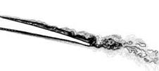
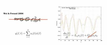
Figure 33 shows an example implementation of the polynomial identifi­cation technique. The DNS computation of a two-dimensional shear-layer, performed by Wei & Freund, is used. The pressure field is sample along the red line shown on the left of the figure. This sampled pressure field is then decomposed using Proper Orthogonal Decomposition, allowing it to be represented in terms of a set of temporal functions, ai(t), and spatial functions, ф(х). Using the polynomial identification technique, truncated to only include the linear term, the coefficients, Lij are determined. The ODE is then integrated in time and the result compared with a truncated rep­resentation (using 40 POD modes, a number found sufficient to reproduce the full DNS field with good accuracy) of the original pressure field.

The integrated ODE, a snapshot of which is shown in figure 33, was found to follow the DNS very closely for about three convective time units. After this the two solutions begin to differ, although the simplified dynamic model continues to behave in a qualitatively similar manner to the DNS.

Bibliography

Reduced Order Modelling

5.2 Introduction

It was shown in section §4 how the analysis tools presented in section §5 can provide a useful means by which the analysis methodology outlined in section §3 can help guide kinematic modelling. However, the final goal, as evoked in the introduction, is to understand and model the dynamic law associated with sound production, as it is only then that one can really claim to have identified source mechanisms.

In this section we provide a very brief introduction to reduced order modelling. For a more complete treatment the reader is encouraged to refer to Noack et al. (2011).

5.3 Two approaches for reduced order dynamical modelling

The governing dynamic law of the full flow system is:

N q = 0. (180)

The objective of reduced order modelling, the final stage of the analysis methodology outlined in section §3, is to construct a simplified dynamic law governing the evolution of a simplified kinematic field, q:

Nq = o. (181)

Two reduced-order dynamic modelling strategies will be outlined here. The first is useful when relatively complete space-time data is available, from a numerical simulation for example, the second being useful in an experimental context, where more limited data is available. In both cases the objective is to write down an Ordinary Differential Equation that mimics either the dynamics of the Navier Stokes operator, or of some reduced sub­space of the system.

This can be achieved once the flow has been expanded in terms of a set of orthogonal basis functions, which can be obtained, for example, by means of POD:[21]

N

q(x, t) = ^2 Oi(t)0(x). (182)

n=1

The temporal evolution of the flow is here contained in a. j(t), and so it is via these, the topos, that we can attempt to write down a simplified

Подпись: do>i dt Подпись: Lij aj + Qijk aj ak : Подпись: (183)

evolution equation, in the form of an ODE:

which mimics both linear and non-linear aspects of the dynamics, via, re­spectively, the first and second terms on the right hand side. The goal is to compute the coefficients, Lij and Qijk, that best reproduce the (known) temporal structure of ai (t); we then have a simplified dynamic model for the flow (or flow sub-space) considered.

The difference between the two said approaches is in the way that the coefficients Lij and Qijk are computed.

Подпись: where Reduced Order Modelling Подпись: (184) (185) (186) (187) (188)

Galerkin projection In this approach, the Navier Stokes equations are projected onto the basis functions, ф(х), giving, directly

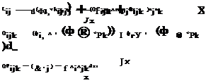
Qijk is here associated with the non-linear convection term of the Navier – Stokes equations, QPjk is associated with the pressure term[22], while Lij is associated with viscous and linear convection terms.

Polynomial identification This technique, proposed by Perret et al. (2006) is useful when only limited experimental data is available. The poly­nomial form

Подпись:Подпись: (189)Lij aj + Qijk aj ak

is chosen as a suitable generic dynamic ansatz; then, knowing the values of ai, we have a linear system of equations with unknowns, Lij and Qijk. By solving this linear system, the coefficients can be identified.

Reduced Order Modelling

Figure 33. Left: instantaneous image of DNS of 2-D mixing-layer of Wei and Freund (2006): pressure fluctuations are sampled along the red line, and this field is then decomposed using POD; Right: green line shows a truncated representation of the DNS solution for the spatial structure of the pressure field on the red line at some given instant in time, while the red line shows the structure predicted by the simplified dynamic model given by the ODE—the quadratic term has been neglected in this example.

Conditional analysis techniques: Stochastic estimation

The following exposition is based on that of Adrian (1996). Consider some variable, q, which is unknown, and another vector quantity E = Ei, i = 1..N which is somehow related to q. We are interested in identifying the functional relationship, q = g(E), which provides some approximation of q in terms of E. This kind of estimation of one variable in terms of another is known as stochastic estimation and is widely used in information theory (Papoulis (1984)). When such a relationship cannot be usefully derived from first principals, we frequently revert to statistics: the joint probability density between q and E is:

/qEdфdф = Prob{-0 < q < ф + dф and ф < E < ф + dф}; (167)

the conditional probability density of q given E is

/q|E (Ф|ф)= /Ч/Е(ф)ф) . (168)

Three estimates of q given E are: (1) the maximum likelihood estimate, defined as the most probable value of q given E, i. e. the value at which /qlE is a maximum; (2) the conditional average of q given E, given by the centroid of the conditional probability

Подпись: (169)< q|E >= J ф/я|Е(ф|фМф;

and, (3) the mean square estimate, i. e. the estimate q = /(E) that min­imises < |q — /(E)| 2 >. It can be shown that the best mean square es­timate of q given E is the conditional average < q|E >. In other words, < |q — /(E)|2 > is a minimum when /(E) =< q|E >.

In this section we outline a technique by which the conditional average can be estimated; in other words we wish to estimate the best estimate: q «< q|E > . The conditional average is approximated by means of a truncated Taylor series expansion about E = 0:

q «<q|E >=/(e) =/(0) + |EЦ + |e2|r + dJL+… (170)

As we do not know the function /(E) we cannot evaluate the derivatives

dn f

dEn and so these are unknowns of the problem. So, considering that the
mean value is zero, (f(0) = 0), the expansion can be written

q «< q|E >= f (E) = AE + BE2 + CE3 + … (171)

and we are required to determine the value of the coefficients A, B, C,… When truncation is performed after the linear term this expression is known as Linear stochastic estimation, when the quadratic term is included we speak of quadratic stochastic estimation, and so on…

Let us now see how to calculate the coefficients, A, in the case where truncation is performed after the linear term. We have

Подпись: (172)q « AE,

Conditional analysis techniques: Stochastic estimation Подпись: (173) (174) (175) (176) (177) (178)

and we would like to obtain a best minimise the error

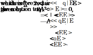
where E has been brought inside the conditional average on account of its being constant with respect to the latter, and, in the final step, the conditional average has been performed over all values of E, reducing the conditional average << qE|E >> to the conventional average < qE >.

Подпись: q Подпись: < qE > E < EE > Подпись: (179)

So, the linear stochastic estimate of q given some related event E, which provides a best approximation to the conditional average < q|E >, is:

This shows the close relationship between the conditional average and the correlation function < qE >. In the context of aeroacoustics, where E is the
radiated acoustic pressure and q the turbulence velocity, such correlations can be shown to provide an approximation to the integral solution of the acoustic analogy (Lee and Ribner (1972)). An example implementation of this technique is provided in section §4.

Koopman modes / Dynamic mode decomposition

The Dynamic Mode Decomposition is a procedure for estimating the eigenvectors and eigenvalues of the Koopman operator. The latter provides a means by which the dynamics of a flow can be analysed, this analysis being effected through some associated observable. An assumption central to the approach is that the flow can be considered as a dynamical system evolving on a manifold D of dimension N. A manifold—the locus of points that comprise the state-space trajectory of a dynamical system—is a gener­alisation, to the non-linear case, of the eigenspace associated with the linear instability of dynamical system in the vicinity of a fixed point : while in a linearised system eigenvectors denote the directions in which that system will move, exponentially, either to or from a fixed point (or equilibrium point), in the non-linear context the manifold amounts to a continuation of these eigenvectors, which continually change direction as the system evolves non-linearly.

This section provides an introduction to both the Koopman operator and the dynamic mode decomposition. The exposition combines elements taken from Rowley et al. (2009), Schmid (2010) and Pastur (2011).

The Koopman operator Let X be a point on D, corresponding to the state of the system at some given time, and let ft be a propagator (frequently referred to as a ‘flow’ or a ‘map’ in dynamical systems or control theory textbooks) that evolves, propagates, or maps, the flow from one time-step to the next; i. e. from X(t0) Є D to X(t0 +1) Є D: 17

X (to +1) = ft {X (to)}. (152)

In an experiment we never have access to the full flow state; at best we may have access to the velocity field on a two-dimensional spatial section (from a PIV measurement for example), with restricted temporal resolution, or single-point information with higher temporal resolution (from a hot-wire, Laser Doppler Velocimeter or microphone for instance). Such an incomplete sample of the flow can be referred to as an observable. We denote this observation by means of a function, q(X), which gives us the observable

7 In the case of fluid flow the propagator is the right hand side of the Navier Stokes equations; i. e. the dynamic law governing the time evolution of the fluid flow.

corresponding to the full state X. q belongs to a Hilbert space, H, and so we can define the norm:

\q\ = v/qqb = у J q2 < ж. (153)

The Koopman operator, Ut, acts in H, such that:

Ut{q(X)} = q(ft[X}). (154)

In other words, the Koopman operator is a map that describes the evolution of the observable, q (which is a function of the full flow state X), from one time-step to the next. The non-linear dynamics associated with the evolu­tion of the full flow leaves its signature in the evolution of the observable; the essence of Koopman/DMD analysis is here: by considering the evolu­tion of the observable we seek to gain insight regarding the nature of the evolution law that underpins the dynamics of the full flow.

The Koopman operator has the following important property. Let фj and Xj be, respectively, eigenfunctions and associated eigenvalues of Ut.[20] If we denote by Xk the state of the system at some time kAt after an initial time t0: Xk = X(to + kAt), then:

The first equality simply corresponds to the definition of the Koopman operator—it evolves the observable, q, from its value when the system is in the state Xk to its value when the system is in the state Xk+1. In the second equality the observable, q, has been expanded in terms of the eigenfunctions of the Koopman operator (chosen here as a suitable set of basis functions); Vj are the associated expansion coefficients, obtained by projecting the ob­servable, q, onto the eigenfunctions, hj. In the third equality the Koopman operator has simply been moved inside the summation, while in the fourth, as hj are eigenfunctions of U, U {hj } can be written as Xjhj.

Vj are the Koopman modes (sometimes referred to as Koopman co­efficients, or dynamic modes), Xj the Koopman eigenvalues and hj the Koopman eigenfunctions. The Dynamic Mode Decomposition constitutes a methodology, similar to the Arnoldi algorithm used in the solution of global stability problems, whereby these quantities can be estimated using limited data sets.

Now, as the evolution of the system from some initial state, Xo to a later state Xk+1 is given by Uк(Xo) (because U(Xk) = UU(Xk-1) = U3(Xk-2) = •••), the state of the observable, q(Xk+1), can be expressed in terms of the state at some initial time, X0, as:

This equation shows that any value of the observable, q, can be deduced from knowledge of the projection of the initial condition q(X0) onto the eigenfunctions, Фі, of the Koopman operator, provided the eigenvalues, Xj are known; this property is important in what follows. Furthermore, if the dynamics considered evolve on a non-degenerated attractor—the dynamics continue to evolve on the manifold, H—then the Koopman operator, U, is a unit operator: the eigenvalues lie on the unit circle and the eigenvectors, Фі, are orthogonal.

Krylov sub-space Consider the following set of successive snapshots of data:

QN-1 = {q(Xo),q(Xi), q(X2), •••, q(XN_i)}, (157)

the sub – and super-scripts on Q indicate the first and last snapshots. Ex­pressed in terms of the Koopman operator this reads:

QN-1 = {q(Xo), U {q(Xo)} , U2 {q(Xo)} , •••, UN-1 {q(Xo)}}, (158)

which is an Ntft-order Krylov subspace. And we know that the Koopman operator applied to this subspace gives:

U {QN-1} = QN : (159)

the action of the Koopman operator is inherently contained in QN.

To this point the observable has been considered a single-point scalar; however, the generalisation to multi-valued observables (for example a ve­locity field obtained from PIV) is straightforward. In this case the Vj are multi-valued and complex.

Dynamic mode decomposition DMD is one possible technique, based on what is known as a companion Matrix, by which the eigenvalues and eigenvectors of U can be estimated; the technique is similar to that used
for the computation of global modes from the Hessenberg matrix using the Arnoldi method.

In what follows we will consider multi-valued observables, represented by the vector q(x, tk). A Krylov subspace is first constructed from sampled data, where the time-step is small enough to resolve all of the dynamics:

Qn-i = {qo, qi, q2,–, qw-i}. (160)

The indices correspond to the successive times, t0,t1,t2, …tN-i. The as­sumption underpinning the companion matrix approach is that the first N fields (where N < M, M being the dimension of the observable q, i. e. the number of spatial points in the snapshot) are sufficient to describe any later realisation of the field q; thus, the Nth snapshot can be expressed as a linear combination of all previous snapshots:

qw = coqo + ciqi + C2q2 + … + cN-iqw-i, (161)

or

qw = QN-ic, (162)

where c = (co, ci, C2,…, cn-i)T and the superscript T denotes hermitian transpose. From equation 158 we know that

u {qN-i} = QN, (163)

i. e. application of the Koopman operator to the Krylov subspace propagates all of the fields by one time-step. In light of this observation, and equation 162, equation 163 can be written as

UQN-i = QN = QN-iC + rT ew, (164)

where C is the companion matrix. eN = (0,0,…, 1)1 Є RN+i and r is a residual vector, orthogonal to the Krylov subspace V0N-i. The residual goes to zero when condition 162 is satisfied.

The following example will help illustrate this. Consider that we have the data:

Подпись: qii qi2 qi3 qi4 q2i q22 q23 q24 q3i q32 q33 q34 Qi

where the first and second indices on the matrix entries denote spatial and temporal coordinates, respectively: each column is a snapshot. We know that the Koopman operator, U, will map from Q3 to Q|:

Подпись: U11 U12 U13' 411 412 413 412 413 414 U21 U22 U23 421 422 423 = 422 423 424 U31 U32 U33_ 431 432 433_ 432 433 434

But, we are also making the assumption that qi4 can be expressed as a linear combination of qi4, qi2 and qi3:

414

C1411 + C2421 + C3431

424

C1412 + C2422 + C3432

434

_C1413 + C2 423 + C3433_

Substituting into the previous equation gives,

U11

U12

U13′

411

412

413

412

413

(C1411 + C2412 + C3413)

U21

U22

U23

421

422

423

422

423

(C1421 + C2422 + C3423)

U31

U32

U33_

431

432

433

_432

433

(C1431 + C2432 + C3433)_

which is the same as

U11

U12

U13′

411

412

413

411

412

413

0

0

C1

U21

U22

U23

421

422

423

421

422

423

1

0

C2

U31

U32

U33_

431

432

433

431

432

433_

0

1

C3

In the more general case, the companion matrix takes the form:

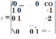
Подпись: /0 ... ... 0 CO 1 0 C1 C = 0 1 C2 . . . 0 � ... 0 1 CN -1 (165)

DMD consists in computing the eigenmodes of the companion matrix, which are then considered as approximations of the eigenmodes of the Koopman operator (when the residual is zero the correspondence is exact). The matrix C has dimension N x N, and its unknown elements, Cj, can be computed by minimising the norm

N-1

qN -^2 cj qj

j=1


min

c


copt


2


Having computed the eigenvalues and eigenvectors of the companion matrix we are finally in a position to write

N

Y,2-1 Фз (Xo)v j.

j=1

The initial conditions фj(X0) are obtained by projecting the initial field, qo, on to the Vj. The eigenfunctions, фj, are Fourier modes, фj = exp(iwjt) if the dynamics are periodic.

The wavelet transform

The wavelet transform provides additional flexibility on two levels when compared with the Fourier transform. (1) The transformed quantity is local in both frequency (or wavenumber) and time (or space); (2) many different kinds of basis function are available, and indeed it is possible to create new functions, provided certain mathematical constraints are satisfied.

The continuous wavelet transform of a signal q(a) is written:

This amounts to the convolution of a signal of interest with a set of wavelet functions ф. This set of functions is generated by dilation and transla­tion of a basic form known as the mother wavelet: dilation is achieved by varying the scale, s, translation being effected by means of the variable, a, which could be a space or time coordinate, for example. The mother wavelet function must satisfy the mathematical constraints of admissibility and regularity; however, provided these constraints are satisfied a good deal of flexibility remains for the design of new mother wavelet functions.

The main difference between the wavelet transform and the Fourier transform is that the former allows space – or time-localised characteristics of a signal to be more clearly identified: the transformed signal is local in both space (and/or time) and scale, whereas its Fourier transformed coun­terpart is local only in frequency, being infinitely extended in space (and/or time).

The following are some relations between the fluctuation energy of a signal, its wavelet transform and its Fourier transform.

1. The relationship between the fluctuation energy, E of the signal q(a) and the wavelet transform of the signal is given by:

E = f q(a)2da = C— f ( |</(s, a)|.|</*(s, a)| dsdda

Jr ф Jr+ J r s2

where Сф is a constant associated with the mother wavelet function used.

2. A global wavelet energy spectrum can be defined as:

egiobai(s) = / e(s, a) da (131)

Jr

where e(s, a) is the energy density as a function of scale, s and the space or time dimension, a.

3. This can also be expressed in terms of the Fourier energy spectrum

E(f ) = W )|2:

egiobai(s) = f E(f)^(sf)|2df (132)

Jr

where ^(sf) is the Fourier transform of the wavelet. This shows that the global wavelet energy spectrum corresponds to the Fourier energy spectrum smoothed by the wavelet spectrum at each scale.

4. The total fluctuation energy of the signal can be obtained by

E = C-1 f eglobal(s)— (133)

JR+* s

5.1 Proper Orthogonal Decomposition

The Proper Orthogonal Decomposition is a data processing technique which is known by this name when used in the field of turbulence anal­ysis, following its introduction for such usage by Lumley (1967). It can also be found referred to as Karhunen-Loeve decomposition, principal com­ponent analysis (Jolliffe (1986)) and singular value decomposition (Golub and Van Loan (1996)). The presentation of POD given here follows that of Delville (1995).

Consider a flow system for which we possess the information q(a, b). The vector q could contain, for example, the values of the three components of velocity on the four-dimensional grid, (x, t); in this case a would represent three-dimensional cartesian space, and b the time direction. We retain the notation a and b in order to keep the derivation as general as possible, because different variants of the POD can be derived from different specific choices of a and b, and associated definitions of the inner product and averaging operations that are applied, respectively, with respect to these coordinates.

POD consists in searching for the function, 0(a), that is best aligned, on average, with the field q(a, b), the averaging operation being with respect to the coordinate b.[19] Both q(a, b) and ф(a) are indefinitely differentiable, have compact support, and belong to the space of square integrable func­tions. The problem is considered in Hibert space, and so it is possible to define the inner product (q, ф)а with respect to a:

л nc /»

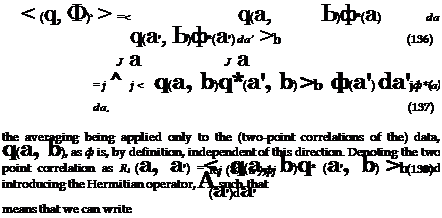
(^Ф)а = q(a, b^*(a) da / qi(a, b)0*(a) da (134)

Л i=i ■’a

where nc denotes the number of components of the vector q (the three components of velocity for example).

The search for the function ф amounts to a search, over the ensemble of realisations of q, for the ф that most closely resembles q on average. This means maximising the projection q(a, b) on the function ф^) with respect to the inner product defined above: we must find the function ф

The wavelet transform

(135)


The wavelet transform

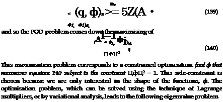
A • фі Mu


(141)


or, in integral form


nc »

У~] / Rij (a, а’)фj (a’) da’ = Лфi(a), j=1a


(142)


The wavelet transform

The wavelet transform

an equation known as the Fredholm integral.

Solution of the integral eigenvalue problem is obtained by means of the theory of Hilbert-Schmidt Lovitt (1950). The details are not given here, but we recall some of the main results:

1. As with most eigenvalue problems, rather than admitting a unique solution, the equation yields a set of solutions:

Подпись: (143)J Щ(a, a’^jn)(a’) da’ = A (п)Ф(п) (a) n = 1, 2, 3,

2. The ensemble of solutions can be chosen such that the eigenfunctions are orthonormal:

[ Ф(Рa)49)(a) da = Spq (144)

J a

3. Any field, qi(a, b), can be expanded in terms of these eigenfunctions, ф(п) (a):

TO

qi(a, b) = £ a(n)(b^n)(a) (145)

n=1

where the coefficients, a(n) (b), are obtained by the projection of qi(a, b) onto ф(п)(a):

a(n) (b) = f qi(a, Ь)Ф(п) (a) da (146)

a

4. The series converges in a least mean square sense and the coefficients, a(n)(b), are mutually uncorrelated:

< a(n) ■ a(m) >= SmnA(n) (147)

5. The eigenvalues are real, positive, their sum finite and they form a convergent series:

A(1) >A(2) > A(3),… (148)

The most common experimental implementation of POD involves space­time velocity or pressure fields: q(a, b) = u(x, t) = u(x, y, z, t) or q(a, b) = p(x, t) = p(x, y,z, t) in which case expansion of the data in terms of the POD eigenfunctions reads

TO

Ui(x, y,z, t) = ^2 a(n)(t)^nx, y,z) (149)

n=1

or (150)

TO

The space-time structure of the measured field is thus separated into spatial (topos) and temporal (chronos) functions. Example implementations are provided in section §4.

The Fourier transform

The Fourier transform is probably the best known and most commonly used data analysis tool in the domain of fluid mechanics and aeroacoustics (and indeed in engineering in general) – the Fourier power spectrum of the sound field radiated by an aeroacoustic system is the quantity that mod­
elling tools are required to reproduce; it is the quantity by which we most often endeavour to assess and understand the behaviour of the system. We recall it briefly in this section, simply so as to have it appear in juxtaposi­tion with a number of alternative, but less commonly used, data-processing tools. We do so because three of the latter (the wavelet transform, Proper Orthogonal Decomposition, and Dynamic Mode Decomposition), as evoked above, bear certain similarities to the Fourier transform in terms of the way their result can be useful as an aid to understanding and modelling; indeed these alternative processing techniques might be best thought of as surrogate tools for assessing complex data in situations where the Fourier transform may not necessarily be the best choice.

The Fourier transform involves the expansion of a given data set in terms of analytical basis functions that are specified a priori; there is no flexibility in this choice. The Fourier transform and its inverse are defined as

Data analysis / reduction

The complexity of most aeroacoustic systems—being associated with high Reynolds number turbulence—means that we frequently find ourselves faced with the task of making sense of large quantities of data; such databases may be the result of numerical simulation and/or experimental measure­ments. Some form of data synthesis, or reduction, is necessary. The data can be considerably compressed, for example, by considering only the time – averaged values of the dependent variables, but at the loss of a large quantity of information. Other time-averaged statistical moments, such as the root mean square (2nd order moment), skewness (3rd order moment) and kur – tosis (4th order moment) can be computed—further information is thereby obtained regarding the state of the system.

Between such time-averaged quantities and the full space-time struc­ture of the system considered there lie many intermediate possibilities for compressing the data into manageable and insight-providing forms. Four techniques by which such intermediate data compression can be obtained (Fourier transform, Wavelet transform, Proper Orthogonal Decomposition and Dynamic Mode Decomposition) are presented in this section, example implementations being found in section §4. Further to these data com – pression/decomposition tools we also present a technique, known as Linear Stochastic Estimation, for the computation of conditional averages. This can constitute a powerful complementary approach when used in conjunc­tion with the said data compression/decomposition tools.

The four data compression techniques discussed have the following com­mon property: they all involve the expansion of space-time data in terms of sets of basis functions. The interest in such an operation is that the very high dimensional flow data can be broken down into a more manageable number of ‘building blocks’, conducive to perspicacious analysis and mod­elling. In the case of spectral and wavelet analyses, the basis functions are analytic and specified a priori; in the case of Proper Orthogonal Decompo­sition the basis functions are empirical and thus intrinsic to the data; in the case of Koopman modes (obtained by Dynamic Mode Decomposition), the functions are associated with the dynamics of the system, in other words they contain information regarding the temporal evolution of the system.