Category THEORETICAL AERODYNAMICS

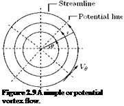
A simple or free vortex is a flow field in which the fluid elements simply translate along concentric circles, without spinning about their own axes. That is, the fluid elements have only translatory motion in a free vortex. In addition to moving along concentric circular paths, if the fluid elements spin about their own axes, the flow field is termed forced vortex.

A simple or free vortex can be established by selecting the stream function, ф, of the source to be the potential function ф of the vortex. Thus, for a simple vortex:

It can be easily shown from Equation (2.42) that the stream function for a simple vortex is:

It follows from Equations (2.42) and (2.43) that the velocity components of the simple vortex, shown in Figure 2.9, are:

Vg = Vr = 0. (2.44)

2 nr

Here again the origin is a singular point, where the tangential velocity Vg tends to infinity, as seen from Equation (2.44). The flow in a simple or free vortex resembles part of the common whirlpool found while paddling a boat or while emptying water from a bathtub. An approximate profile of a whirlpool is as shown in Figure 2.10. For the whirlpool, shown in Figure 2.10, the circulation along any path about the origin is given by:

Г = ф V ■ dl

/* 2n

Vgrdg.

0

z

Since there are no other singularities for the whirlpool, shown in Figure 2.10, this must be the circulation for all paths about the origin. Consequently, q in the case of vortex is the measure of circulation about the origin and is also referred to as the strength of the vortex.

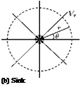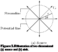
Source is a potential flow field in which flow emanating from a point spreads radially outwards, as shown in Figure 2.8(a). Sink is potential flow field in which flow gushes towards a point from all radial directions, as illustrated in Figure 2.8(b).

Consider a source at origin, shown in Figure 2.8(a). The volume flow rate q crossing a circular surface of radius r and unit depth is given by:

q = 2nrVr, (2.38)

where Vr is the radial component of velocity. The volume flow rate q is referred to as the strength of the source. For a source, the radial lines are streamlines. Therefore, the potential lines must be concentric circles, represented by:

ф = A ln(r), (2.39)

where A is a constant. The radial velocity component Vr = дф/dr = A/r.

Substituting this into Equation (2.39), we get:

2nrA

—— = q

r

or

A = ±.

2n

Thus, the velocity potential for a two-dimensional source of strength q becomes:

In a similar manner as above, the stream function for a source of strength q can be obtained as:

where в is the orientation (inclination) of the streamline from the x-direction, measured in the counter­clockwise direction, as shown in Figure 2.8(a). Similarly, for a sink, which is a type of Bow in which the fluid from infinity flows radially towards the origin, we can show that the potential and stream functions are given by:

where q is the strength of the sink. Note that the volume flow rate is termed the strength of source and sink. Also, for both source and sink the origin is a singular point.

Potential flow is based on the concept that the flow field can be represented by a potential function ф such that:

(2.35)

This linear partial differential equation is popularly known as Laplace equation. Derivatives of ф with respect to the space coordinates x, y and z give the velocity components Vx, Vy and Vz, respectively, along x-, y – and z – directions. Unlike the stream function ф, the potential function can exist only if the flow is irrotational, that is, when viscous effects are absent. All inviscid flows must satisfy the irrotationality condition:

(2.36)

For two-dimensional potential flows, by Equation (2.30), we have the vorticity Z as:

dV dV

Zz = — —x = 0.

dx dy

Using Equation (2.33), we get the vorticity as:

This shows that the flow is irrotational. For two-dimensional incompressible flows, the continuity equation is:

V V =

dx dy

In terms of the potential function ф, this becomes:

d2 ф d2 ф

—— – I—— = 0

dx2 dy2

that is:

V2ф = 0.

This linear equation is the governing equation for potential flows. For potential flows, the Navier-Stokes equations (2.23) reduce to:

Equation (2.37) is known as Euler’s equation.

At this stage, it is natural to have the following doubts about the streamline and potential function, because we defined the streamline as an imaginary line in a flow field and potential function as a mathe­matical function, which exists only for inviscid flows. The answers to these vital doubts are the following:

• Among the graphical representation concepts, namely the pathline, streakline and streamline, only the first two are physical, and the concept of streamline is only hypothetical. But even though imaginary, the streamline is the only useful concept, because it gives a mathematical representation for the flow field in terms of stream function ф, with its derivatives giving the velocity components. Once the velocity components are known, the resultant velocity, its orientation, the pressure and temperature associated with the flow can be determined. Thus, streamline plays a dominant role in the analysis of fluid flow.

• Knowing pretty well that no fluid is inviscid or potential, we introduce the concept of potential flow, because this gives rise to the definition of potential function. The derivatives of potential function with the spatial coordinates give the velocity components in the direction of the respective coordinates and the substitution of these velocity components in the continuity equation results in Laplace equation. Even though this equation is the governing equation for an impractical or imaginary flow (inviscid flow), the fundamental solutions of Laplace equation form the basis for both experimental and computational flow physics. The basic solutions for the Laplace equation are the uniform flow, source, sink and free or potential vortex. These solutions being potential can be superposed to get the mathematical functions representing any practical geometry of interest. For example, superposition of a doublet (source and a sink of equal strength in proximity) and uniform flow would represent flow past a circular cylinder. In the same manner, suitable distribution of source and sink along the camberline and superposition of uniform flow over this distribution will mathematically represent flow past an aerofoil. Thus, any practical geometry can be modeled mathematically, using the basic solutions of the Laplace equation.

Streamlines are imaginary lines in the flow field such that the velocity at all points on these lines are always tangential to them. Flows are usually depicted graphically with the aid of streamlines. Streamlines proceeding through the periphery of an infinitesimal area at some time t forms a tube called streamtube, which is useful for the study of fluid flow phenomena. From the definition of streamlines, it can be inferred that:

• Flow cannot cross a streamline, and the mass flow between two streamlines is conserved.

• Based on the streamline concept, a function ф called stream function can be defined. The velocity components of a flow field can be obtained by differentiating the stream function.

In terms of stream function ф, the velocity components of a two-dimensional incompressible flow are given as:

It is important to note that the stream function is defined only for two-dimensional flows, and the definition does not exist for three-dimensional flows. Even though some books define ф for axisymmetric flow, they again prove to be equivalent to two-dimensional flow. We must realize that the definition of ф does not exist for three-dimensional flows, because such a definition demands a single tangent at any point on a streamline, which is not possible in three-dimensional flows.

2.8.1 Relationship between Stream Function and Velocity Potential

For irrotational flows (the fluid elements in the field are free from rotation), there exists a function ф called velocity potential or potential function. For a steady two-dimensional flow, ф must be a function of two space coordinates (say, x and y). The velocity components are given by:

From Equations (2.31) and (2.33), we can write:

(2.34)

These relations between stream function and potential function, given by Equation (2.34), are the famous Cauchy-Riemann equations of complex-variable theory. It can be shown that the lines of constant ф or potential lines form a family of curves which intersect the streamlines in such a manner as to have the tangents of the respective curves always at right angles at the point of intersection. Hence, the two sets of curves given by ф = constant and ф = constant form an orthogonal grid system or flow-net. That is, the streamlines and potential lines in flow field are orthogonal.

Unlike stream function, potential function exists for three-dimensional flows also, because there is no condition like the local flow velocity must be tangential to the potential lines imposed in the definition of ф. The only requirement for the existence of ф is that the flow must be potential.

When a fluid element is subjected to a shearing force, a velocity gradient is produced perpendicular to the direction of shear, that is, a relative motion occurs between two layers. To encounter this relative motion the fluid elements have to undergo rotation. A typical example of this type of motion is the motion between two roller chains rubbing each other, but moving at different velocities. It is convenient to use an abstract quantity called circulation Г, defined as the line integral of velocity vector between any two points (to define rotation of the fluid element) in a flow field. By definition:

where dl is an elemental length, c is the path of integration.
Circulation per unit area is known as vorticity Z,

Z = Г/A.

In vector form, Z becomes:

where V is the flow velocity, given by V = i Vx + j Vy, and:

d d

V = i——- + j —.

dx dy

For a two-dimensional flow in xy-plane, vorticity Z becomes:

dVL_dV1

z dx dy

where Zz is the vorticity about the z-direction, which is normal to the flow field. Likewise, the other components of vorticity about x – and y-directions are:

_ dVz dVy

Zx ^ …

dy dz xz

y dz dx

If Z = 0, the flow is known as irrotational Bow. Inviscid flows are basically irrotational flows.

Transition point may be defined as the end of the region at which the flow in the boundary layer on the surface ceases to be laminar and begins to become turbulent. It is essential to note that the transition from laminar to turbulent nature takes place over a length, and not at a single point. Thus the transition point marks the beginning of the transition process from laminar to turbulent nature.

2.7.2 Separation Point

Separation point is the position at which the boundary layer leaves the surface of a solid body. If the separation takes place while the boundary layer is still laminar, the phenomenon is termed laminar separation. If it takes place for a turbulent boundary layer it is called turbulent separation.

The boundary layer theory makes use of Navier-Stokes Equation (2.23) with the viscous terms in it but in a simplified form. On the basis of many assumptions such as, boundary layer thickness is small compared to the body length and similarity between velocity profiles in a laminar flow, the Navier-Stokes equation can be reduced to a nonlinear ordinary differential equation, for which special solutions exist. Some such problems for which Navier-Stokes equations can be reduced to boundary layer equations and closed form solutions can be obtained are: flow past a flat plate or Blassius problem; Hagen-Poiseuille flow through pipes; Couette flow between a stationary and moving parallel plates; and flow between rotating cylinders.

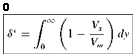
Displacement thickness S* may be defined as the distance by which the boundary would have to be displaced if the entire flow field were imagined to be frictionless and the same mass flow is maintained at any section.

Consider unit width in the flow over an infinite flat plate at zero angle of incidence, and let the x – component of velocity to be Vx and the у-component of velocity be Vy. The volume flow rate Aq through this boundary layer segment of unit width is given by:

Aq = (Vm – Vx) dy,

0

where Vm is the main stream (frictionless flow) velocity component and Vx is the actual local velocity component. To maintain the same volume flow rate q for the frictionless case, as in the actual case, the boundary must be shifted out by a distance S* so as to cut off the amount Aq of volume flow rate. Thus:

•TO

(2.24)

The displacement thickness is illustrated in Figure 2.7. The main idea of this postulation is to permit the use of a displaced body in place of the actual body such that the frictionless mass flow around the displaced body is the same as the actual mass flow around the real body. The displacement thickness concept is made use of in the design of wind tunnels, air intakes for jet engines, and so on.

The momentum thickness в and energy thickness Se are other (thickness) measures pertaining to bound­ary layer. They are defined mathematically as follows:

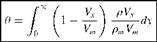(2.25)

_L

b

x

Hypothetical flow with displaced boundary

Figure 2.7 Illustration of displacement thickness.

where Vm and pm are the velocity and density at the edge of the boundary layer, respectively, and Vx and p are the velocity and density at any y location normal to the body surface, respectively. In addition to boundary layer thickness, displacement thickness, momentum thickness and energy thickness, we can define the transition point and separation point also with the help of boundary layer.

A closer look at the essence of the displacement, momentum and energy thicknesses of a boundary layer will be of immense value from an application point of view. First of all, S*, в and Se are all length parame­ters, in the direction normal to the surface over which the boundary layer prevails. Physically, they account for the defect in mass flow rate, momentum and kinetic energy, caused by the viscous effect. In other words:

• The displacement thickness is the distance by which the boundary, over which the boundary layer prevails, has to be hypothetically shifted, so that the mass flow rate of the actual flow through distance S and the ideal (inviscid) flow through distance (S — S*), illustrated in Figure 2.7, will be the same.

• The momentum thickness is the distance by which the boundary, over which the boundary layer prevails, has to be hypothetically shifted, so that the momentum associated with the mass passing through the actual thickness (distance) S and the hypothetical thickness (S — в) will be the same.

• The energy thickness is the distance by which the boundary, over which the boundary layer prevails, has to be hypothetically shifted, so that the kinetic energy of the flow passing through the actual thickness (distance) S and the hypothetical thickness (S — Se) will be the same.

Kinematics is the branch of physics that deals with the characteristics of motion without regard for the effects of forces or mass. In other words, kinematics is the branch of mechanics that studies the motion of a body or a system of bodies without consideration given to its mass or the forces acting on it. It describes the spatial position of bodies or systems, their velocities, and their acceleration. If the effects of forces on the motion of bodies are accounted for the subject is termed dynamics. Kinematics differs from dynamics in that the latter takes these forces into account.

To simplify the discussions, let us assume the flow to be incompressible, that is, the density is treated as invariant. The basic governing equations for an incompressible flow are the continuity and momentum equations. The continuity equation is based on the conservation of matter. For steady incompressible flow, the continuity equation in differential form is:

where Vx, Vy and Vz are the velocity components along x-, y – and z-directions, respectively. Equation (2.22) may also be expressed as:

V – V = 0,

V = i — + j— + k —

dx dy dz

and V = iVx + jVy + kVz.

The momentum equation, which is based on Newton’s second law, represents the balance between various forces acting on a fluid element, namely:

1. Force due to rate of change of momentum, generally referred to as inertia force.

2. Body forces such as buoyancy force, magnetic force and electrostatic force.

3. Pressure force.

4. Viscous forces (causing shear stress).

For a fluid element under equilibrium, by Newton’s second law, we have the momentum equation as:

For a gaseous medium, body forces are negligibly small compared to other forces and hence can be neglected. For steady incompressible flows, the momentum equation can be written as:

dVx dVx dVx

Vx —x + Vy —- + Vz —- =

dx y dy dz

Equations (2.23a), (2.23b), (2.23c) are the x, y, z components of momentum equation, respectively. These equations are generally known as Navier-Stokesequations. They are nonlinear partial differential equations and there exists no known analytical method to solve them. This poses a major problem in fluid flow analysis. However, the problem is tackled by making some simplifications to the equation, depending on the type of flow to which it is to be applied. For certain flows, the equation can be reduced to an ordinary differential equation of a simple linear type. For some other type of flows, it can be reduced to a nonlinear ordinary differential equation. For the above types of Navier-Stokes equation governing special category of flows, such as potential flow, fully developed flow in a pipe or channel, and boundary layer over flat plates, it is possible to obtain analytical solutions.

It is essential to understand the physics of the flow process before reducing the Navier-Stokes equations to any useful form, by making appropriate approximations with respect to the flow. For example, let us examine the flow over an aircraft wing, shown in Figure 2.4.

This kind of problem is commonly encountered in fluid mechanics. Air flow over the wing creates higher pressure at the bottom, compared to the top surface. Hence, there is a net resultant force component normal to the freestream flow direction, called lift, L, acting on the wing. The velocity varies along the wing chord as well as in the direction normal to its surface. The former variation is due to the shape of the aerofoil, and the latter is due to the no-slip condition at the wall. In the direction normal to wing surface, the velocity gradients are very large in a thin layer adjacent to the surface and the flow reaches asymptotically to the freestream velocity within a short distance, above the surface. This thin

region adjacent to the wall, where the velocity increases from zero to freestream value, is known as the boundary layer. Inside the boundary layer the viscous forces are predominant. Further, it so happens that the static pressure outside the boundary layer, acting in the direction normal to the surface, is transmitted to the boundary through the boundary layer, without appreciable change. In other words, the pressure gradient across the boundary layer is zero. Neglecting the inter-layer friction between the streamlines, in the region outside the boundary layer, it is possible to treat the flow as inviscid. Inviscid flow is also called potential Bow, and for this case the Navier-Stokes equation can be simplified to become linear. It is possible to obtain the pressures in the field outside the boundary layer and treat this pressure to be invariant across the boundary layer, that is, the pressure in the freestream is impressed through the boundary layer. For low-viscous fluids such as air, we can assume, with a high degree of accuracy, that the flow is frictionless over the entire flow field, except for a thin region near solid surfaces. In the vicinity of solid surface, owing to high velocity gradients, the frictional effects become significant. Such regions near solid boundaries, where the viscous effects are predominant, are termed boundary layers.

In general, boundary layer over streamlined bodies are extremely thin. There may be laminar and turbulent flow within the boundary layer, and its thickness and profile may change along the direction of the flow. Consider the flow over a flat plate shown in Figure 2.5. Different zones of boundary layer over a flat plate are shown in Figure 2.5. The laminar sublayer is that zone adjacent to the boundary, where the turbulence is suppressed to such a degree that only the laminar effects prevail. The various regions shown in Figure 2.5 are not sharp demarcations of different zones. There is actually a gradual transition from one region, where certain effect predominates, to another region, where some other effect is predominant.

Although the boundary layer is thin, it plays a vital role in fluid dynamics. The drag on ships, aircraft and missiles, the efficiency of compressors and turbines of jet engines, the effectiveness of ramjets and turbo­jets, and the efficiencies of numerous other engineering devices, are all influenced by the boundary layer to a significant extent. The performance of a device depends on the behavior of boundary layer and its effect on the main flow. The following are some of the important parameters associated with boundary layers.

2.7.1 Boundary Layer Thickness

Boundary layer thickness S may be defined as the distance from the wall in the direction normal to the wall surface, where the fluid velocity is within 1% of the local main stream velocity. It may also be

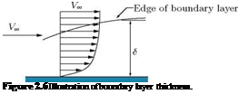defined as the distance S, normal to the surface, in which the flow velocity increases from zero to some specified value (for example, 99%) of its local main stream flow velocity. The boundary layer thickness S may be shown schematically as in Figure 2.6.

The analysis in which large control volumes are used to obtain the aggregate forces or transfer rates is termed integral analysis. When the analysis is applied to individual points in the flow field, the resulting equations are differential equations, and the method is termed differential analysis.

2.6.2 State Equation

For air at normal temperature and pressure, the density p, pressure p and temperature T are connected by the relation p = pRT, where R is a constant called gas constant. This is known as the thermal equation of state. At high pressures and low temperatures, the above state equation breaks down. At normal pressures and temperatures, the mean distance between molecules and the potential energy arising from their attraction can be neglected. The gas behaves like a perfect gas or ideal gas in such a situation. At this stage, it is essential to understand the difference between the ideal and perfect gases. An ideal gas is frictionless and incompressible. The perfect gas has viscosity and can therefore develop shear stresses, and it is compressible according to state equation.

Real gases below critical pressure and above the critical temperature tend to obey the perfect-gas law. The perfect-gas law encompasses both Charles’ law and Boyle’s law. Charles’ law states that at constant pressure the volume of a given mass of gas varies directly as its absolute temperature. Boyle’s law (isothermal law) states that for constant temperature the density varies directly as the absolute pressure.

In the range of engineering interest, four basic laws must be satisfied by any continuous medium. They are:

• Conservation of matter (continuity equation).

• Newton’s second law (momentum equation).

• Conservation of energy (first law of thermodynamics).

• Increase of entropy principle (second law of thermodynamics).

In addition to these primary laws, there are numerous subsidiary laws, sometimes called constitutive relations, that apply to specific types of media or flow processes (for example, equation of state for perfect gas, Newton’s viscosity law for certain viscous fluids, isentropic and adiabatic process relations are some of the commonly used subsidiary equations in flow physics).

2.6.1 System and Control Volume

In employing the basic and subsidiary laws, any one of the following modes of application may be adopted:

• The activities of each and every given element of mass must be such that it satisfies the basic laws and the pertinent subsidiary laws.

• The activities of each and every elemental volume in space must be such that the basic laws and the pertinent subsidiary laws are satisfied.

In the first case, the laws are applied to an identified quantity of matter called the control mass system. A control mass system is an identified quantity of matter, which may change shape, position, and thermal condition, with time or space or both, but must always entail the same matter.

For the second case, a definite volume called control volume is designated in space, and the boundary of this volume is known as control surface. The amount and identity of the matter in the control volume may change with time, but the shape of the control volume is fixed, that is, the control volume may change its position in time or space or both, but its shape is always preserved.