Category Basics of Aero – thermodynamics

The topic of laminar-turbulent transition was given much room in this chap­ter. This was deemed to be necessary because of its large importance for hypersonic vehicle design.

A definitive improvement of the capabilities to predict laminar-turbulent transition, but also to optimize surface shapes in order to, for instance, delay transition, is mandatory for CAV’s as well as for ARV’s. Vehicles of these classes are viscous-effect dominated, which—as was discussed and shown in several of the preceding chapters—regards the thermal state of the surface, thermal surface effects, the drag of the vehicle, the thermal loads in view of the structure and materials concept of the vehicle, and issues of aerothermo – dynamic propulsion integration.

For RV’s the improvement of transition prediction is highly desirable, too, because the effectiveness of these vehicles must be improved by minimizing the mass of the thermal protection system. In this regard laminar-turbulent
transition on the lower branch of the re-entry trajectory, as well as on alter­native lower altitude trajectories than preferred today, including contingency trajectories, is of great importance and demands a more accurate and reliable prediction than is possible today.

The general knowledge about transition phenomena in high-speed flows is already rather good, and the development of new prediction methods is en­couraging. Here non-local and non-linear theory appears to have the necessary potential. In the not too far future the use of such methods in aerothermody – namic numerical simulations and optimizations also in industrial design work will be no problem in view of the still strongly growing computer capabilities.

Necessary to achieve the improvements of transition prediction is con­tinuous concerted research, extension and use of “quiet” ground-simulation facilities, and in-flight measurements on ad-hoc experimental vehicles or in passenger experiments on other vehicles. Ground and flight measurements need also the careful recording of the thermal state of the surface by means of a suitable hot experimental technique. A combination of analytical work, computational simulation, ground-facility simulation, and in-flight simula­tion (unified approach [143]), in a transfer-model ansatz, which takes also into account—where necessary—the coupling of the flow to the vehicle sur­face, is considered to be necessary, in order to advance this scientifically and technically fascinating and challenging field [3].

In the last two decades the knowledge of instability and transition phenom­ena has increased considerably, and many new and comprehensive stabil- ity/instability methods are now available. However, the accurate and reliable prediction of the shape, the extent and the location of the transition zone, i. e., the transition sub-branch IIb, Fig. 8.1, for real flight vehicles of the ve­hicle classes considered here is not possible.[147] This holds partly also for flows in the other speed regimes. Thus when we speak about transition prediction it is in the sense of transition estimation.

We distinguish three classes of means for transition prediction, namely

— non-empirical,

— semi-empirical,

— empirical

methods and criteria. Of these the latter two rely partly or fully on experi­mental data.

The major problem is that all-encompassing high-speed experimental data bases still are very scarce. These, in principle, could come either from ground – simulation facilities or from free-flight measurements. For the first it is noted that a hypersonic ground-simulation facility is not able to duplicate the at­mospheric flight environment and also not the relevant boundary-layer prop­erties, i. e., the profiles of the tangential velocity, the temperature and the density normal to the surface in presence of radiation cooling, as they are present on a real vehicle’s surface [7].

This holds especially for regular but also for forced transition. With regard to free-flight measurements we must observe that the available transition data sets obtained at actual high-speed flight, see, e. g., [106], are not always the necessary multi-parametric data bases, which are required to identify the major instability and transition phenomena involved, including the relevant flow and surface properties.

We give now a short overview over the three classes of methods and criteria for transition prediction, for the first two classes see also the review [101]. Regarding semi-empirical and empirical methods and criteria we note that it is necessary for a given practical application to make first a thorough assessment of the flow field under consideration as was done for instance in

Section 1.2. The data base underlying the method or criterion to be employed must correspond as accurately as possible to the considered flow field.

Non-empirical Transition Prediction. It appears that non-local non­linear instability methods have the real potential to become in the long term the needed non-empirical transition prediction methods for practical pur­poses. Direct numerical simulation (DNS) as well as large eddy simulation (LES), due to the needed very large computer power, will have, for a long time to come, their domain of application in numerical experiments of re­search only.

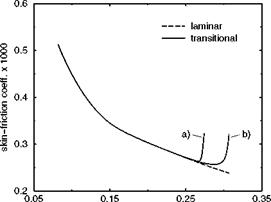
The present state of development of non-local non-linear methods ap­pears to permit the prediction of the location of stage 5, i. e., the beginning of sub-branch IIb, as for instance is demonstrated by Fig. 8.12 [43]. However, two different combinations of disturbance modes—a) and b)—lead to small, but significant differences between the solutions (location and initial shape of sub-branch IIb). This points to the problem of handling free-stream distur­bances, Sub-Section 8.3.2, which still is a major obstacle for the non-empirical transition prediction.

The result of Fig. 8.12 is for a low-speed case, similar results for the high­speed flows of interest are available to a certain extent. It can be expected, in view of the references given in Sub-Section 8.4.1, that at least results similar to those shown can be obtained, after additional research has been conducted, especially also with regard to the receptivity problem [101].

Very encouraging is in this context that the problem of surface irregulari­ties (transition triggering, permissible properties) seems to become amenable for non-empirical prediction methods, see [130], at least for transonic flow past swept wings.[148] That would allow to take into account the influence of weak surface irregularities on regular transition, but also to model transition forced, for example, by the rough tile surface of a TPS.

Semi-empirical Transition Prediction. Semi-empirical transition pre­diction methods go back to J. L. van Ingen [132], and A. M.O. Smith and N. Gamberoni [133]. They observed independently in the frame of local linear stability theory that, for a given boundary-layer mean flow, the envelope of the most amplified disturbances, see Fig. 8.7 for (two) examples, correlates observed transition locations.

For airfoils it turned out, that on average the value, see Sub-Section 8.1.2,

A t

In — = Midi = 9, (8.31)

A0 Jt о

best correlates the measured data, hence the name e9 criterion. Unfortunately later the “universal constant” 9 turned out to be a “universal variable”. Already in the data base of Smith and Gamberoni the scatter was up to 20 per cent. Now we speak of the en criterion, which for well defined flow classes with good experimental data bases can be a reliable and accurate transition prediction tool, see, e. g., [134]. The disturbance environment can be regarded to some degree. The free-stream turbulence Tu of a wind tunnel, for instance, can be taken into account by introducing ntr = ntr (Tu) [135]. Surface roughness can be treated, too.

The en method can be used by employing the parabolized stability equa­tions (PSE) approach [19]. The result is a linear, non-local method. With this method surface curvature and non-parallel effects can be taken into account.

For three-dimensional flows the situation becomes complicated, see, e. g., [107]. Non-local linear stability theory with n-factors for Tollmien-Schlichting modes (nTS) and for cross-flow modes (nCF), based on in-flight measured data, are used increasingly in transonic swept-wing flows, see the discussion in [28].

Although the en method does not describe at least the initial stage of tran­sition, i. e., the beginning of sub-branch IIb, it has been extensively applied to mainly two-dimensional high-speed flows [11, 134, 57]. It is a valuable tool to study instability phenomena and their influence on transition, but also to perform parametric studies. To reliably predict transition on hypersonic flight vehicles is primarily a matter of a reliable, all-encompassing multi-parametric experimental data base, which is not available. To question is also whether an en method permits to treat the effect of weak surface irregularities on regular transition, but also to describe forced transition. In [101] en methods
are seen as intermediate step along the way to non-empirical methods—there called mechanism-based methods—in hypersonic flows.

Empirical Transition Prediction. Empirical transition prediction is based on criteria derived from experimental data which are obtained in ground- simulation facilities but also in free flight. Such criteria have been applied and are applied in the design of the Space Shuttle Orbiter, of BURAN, of re-entry bodies, launchers, and missiles.

The empirical criteria usually are local criteria, i. e., they employ local integral boundary-layer and boundary-layer edge-flow properties. This means that all the phenomena discussed in Sub-Sections 8.1.3 to 8.2.9 are not taken into account explicitly. At best some of them are implicitly regarded via an employed boundary-layer integral quantity. Data from ground-simulation facilities are possibly falsified by tunnel noise effects. The lower (xtr, i) and the upper (xtr, u) transition location often are not explicitly given, i. e., length and shape of the transition sub-branch IIb, Fig. 8.1, are not specified. This holds also for the overshoot at the end of this branch.

Due to the nature of the criteria, the predictions based on them are of questionable quality. If error bars are given, uncertainties of describing data and hence design margins can be established. In any case parametric guesses can be made.

Empirical criteria are discussed in depth in, for instance, [11] and [57]. In [57] available high-speed flow criteria, in this case basically two-dimensional criteria, are grouped into four classes:

— Smooth body criteria, i. e., criteria to predict regular transition. A typical criterion from this class is the Thyson criterion [136]:

Res2,tr = 200 e0187 Me. (8.32)

Reg2 tr is the Reynolds number based on the boundary-layer edge data and the momentum thickness S2, Me is the edge Mach number. The correla­tion data are mainly from ground-simulation facilities and hence the noise problem exists.

To this class of criteria also the criterion by H. W. Kipp and R. V. Masek is counted [137]. Written in the general form

it can be applied to different configurations, although it was originally developed for the Space Shuttle Orbiter design. Stetson [11] discusses this criterion in detail and states that it cannot be applied in general.

— Rough body criteria, i. e., criteria to predict transition forced by single or distributed (TPS surface) roughnesses. As example a criterion for dis­tributed roughness, developed in the frame of the HERMES project with data from Space Shuttle Orbiter flights, is given [138, 57]:

The corrected roughness height kcorr is defined by

The roughness is efficient if located less than 6 m from the vehicle nose and k/S1 = 0.1 to 0.5.

The criterion takes into account the roughness height k, the boundary-layer edge data pe, ue, pe, the displacement thickness Ji, the boundary-layer edge Mach number Me, and the longitudinal curvature R. It is defined for the lower symmetry line of the vehicle and duplicates well the Space Shuttle Orbiter data there. The need for a truly three-dimensional approach is acknowledged by the authors.

— Combined rough/smooth body criteria, i. e., criteria with parameters to distinguish sub-critical and super-critical roughness regimes. An example is the criterion given by W. D. Goodrich et al. in order to improve the transition prediction for the Space Shuttle Orbiter [2].

— Global criteria take into account implicitly all phenomena of interest for a given vehicle class. In [139], for instance, data are correlated for ballistic re-entry vehicles with ablative nose tips, however with mixed success.

More recent publications regarding ground facility and flight data can be found in [42, 106] and [140]-[142].

Criteria, which take into account effects of three-dimensionality, for in­stance, cross-flow instability or attachment-line contamination are discussed too in [57]. We have treated them in Section 8.2.

In this section we wish to acquaint the reader with the possibilities to ac­tually predict stability/instability and transition in high-speed flows. No re­view is intended, but a general overview is given with a few references to prediction models and criteria. Because many developments in non-local and non-linear instability prediction were mainly made for transonic flows, these developments will be treated too in order to show their potential also for the high-speed flows of interest here. Transition-prediction theory and methods based on experimental data (ground-simulation facility or free-flight data) are treated under the headings “semi-empirical” and “empirical” transition prediction in Sub-Section 8.4.2. Transition prediction for high-speed flows generally has made much progress in the last decade, although the ultimate goal still is to be achieved. The review paper [101] and the overview paper on AFOSR-sponsored research in aerothermodynamics [79] are good intro­ductions to the present state of the art. For a review of flight data regarding laminar-turbulent transition in high-speed flight see, e. g., [106].

8.4.1 Stability/instability Theory and Methods

Theory and methods presented here are in any case methods for compressible flow but not necessarily for flow with high-temperature real-gas effects. The thermal boundary conditions are usually only the constant surface tempera­ture or the adiabatic-wall condition. The radiation-adiabatic wall condition is implemented only in few methods, although it is in general straight forward to include it into a method. Likewise, it is not a problem to include adequate high-temperature real-gas models into stability/instability methods.

Linear and Local Theory and Methods. The classical stability theory is a linear and local theory. It describes only the linear growth of disturbances (stage 2—see the footnote on page 284—in branch IIa, Fig. 8.1). Neither the receptivity stage is covered, nor the saturation stage and the last two stages of transition.[146] Extensions to include non-parallel effects are possible and have been made. The same is true for curvature effects. However, the suitability of such measures appears to be questionable, see, e. g., [107].

Linear and local theory is, despite the fact that it covers only stage 2, the basis for the semi-empirical en transition prediction methods, which are discussed in Sub-Section 8.4.2.

Linear and local stability methods for compressible flows are for instance COSAL (M. R. Malik, 1982 [108]), COSTA (U. Ehrenstein and U. Dall – mann, 1989 [109]), COSMET (M. Simen, 1991 [110], see also E. Kufner [34]), CASTET (F. Laburthe, 1992 [111]), SHOOT (A. Hanifi, 1993 [112]), LST3D (M. R. Malik, 1997 [113]), COAST (G. Schrauf, 1992 [114], 1998 [115]), LILO (g. Schrauf, 2004 [116]).

Non-local Linear and Non-linear Theory and Methods. Non-local theory takes into account also the downstream changes of the mean flow as well as the changes of the amplitudes of the disturbance flow and the wave numbers. Non-local and linear theory also describes only stage 2 in branch IIa, Fig. 8.1. However, non-parallel effects and curvature effects are consistently taken into account which makes it a better basis for en methods than local linear theory.

Non-linear non-local theory on the other hand describes all five stages, in particular also stage 1, the disturbance reception stage, however not in all respects. Hence, in contrast to linear theory, form and magnitude of the initial disturbances must be specified, i. e., a receptivity model must be employed, Sub-Section 8.3.

Non-local methods are (downstream) space-marching methods that solve a system of disturbance equations, which must have space-wise parabolic character. Hence such methods are also called “parabolized stability equa­tions (PSE)” methods. We do not discuss here the parabolization and solution strategies and refer the reader instead to the review article of Th. Herbert [117] and to the individual references given in the following.

Non-local linear stability methods for compressible flow are for instance xPSE (F. P. Bertolotti, linear and non-linear (the latter incompressible only), 1991 [118]), PSE method (linear and non-linear) (C.-L. Chang et al., 1991 [119]), NOLOS (M. Simen, 1993 [120]), PSE-Chem (H. B. Johnson et al., 2005 [121]), STABL-3D (H. B. Johnson et al., 2010 [122]).

Non-local non-linear stability methods for compressible flow are for in­stance, COPS (Th. Herbert et al., 1993 [123]), NOLOT/PSE (M. Simen et al., 1994 [124], see also S. Hein [43]), CoPSE (M. S. Mughal and P. Hall, 1996 [125]), PSE3D (M. R. Malik, 1997 [113], with chemical reactions also see [126]), xPSE with rotational and vibrational non-equilibrium (F. P. Bertolotti, 1998 [63]), NELLY (H. Salinas, 1998 [127]), LASTRAC (C.-L. Chang, 2004 [128]), JoKHeR (J. J. Kuehl et al., 2012 [129]).

Under environment we understand either the atmospheric flight environment of a hypersonic flight vehicle or the environment which the sub-scale model of the flight vehicle has in a ground-simulation facility. The question is how the respective environment influences instability and transition phenomena on the flight vehicle or on its sub-scale model [15, 92]. Ideally there should be no differences between the flight environment and the ground-facility en­vironment, but the fact that we have to distinguish between these two envi-

ronments already points to the fact that these environments have different characteristics and different influences on transition. These different influ­ences pose large problems both in view of scientific topics and practical, i. e., vehicle design issues.

The atmosphere, through which a hypersonic vehicle flies, constitutes a disturbance environment. Information about the environment appears to be available for the troposphere, but not so much for the stratosphere, Fig. 2.1. Morkovin suggests, [12], see also [13], as a work hypothesis, that distribution, intensities and scales of disturbances can be assumed to be similar in the troposphere and the stratosphere. Flight measurements in the upper tropo­sphere (11 km altitude) have shown strong anisotropic air motions with very low dissipation and weak vertical velocity fluctuations [93]. How much the flight speed of the vehicle plays a role is not known. This partly will be a matter of the receptivity properties of the boundary layer.

Much is known of the disturbance environment in ground-simulation facil­ities, see, e. g., [11]—[14]. We have mentioned already as major problem noise, i. e., the sound field radiated from the turbulent boundary layers of the tun­nel wall.[143] The quest to create in ground-simulation facilities a disturbance environment similar to that of free flight (whatever that is, see in this regard also [94]) has led to the concept of the “quiet” tunnel, see, e. g., [13].

A Mach 3.5 pilot quiet tunnel has been built in the 1970s in the US at NASA Langley [95]. It is characterized by measures to remove the tur­bulent boundary layer coming from the settling chamber, a new boundary layer developing on the nozzle wall, and finally a sound shield (effectiveness?) enclosing the test section.

The Ludwieg-Tube facilities at the DLR in Gottingen, and at the Tech­nical University Braunschweig, Germany, see, e. g., [96], as well as the Weise – Tube facility of similar principle at the University Stuttgart [97], can not be considered as quiet tunnels. At least the unit Reynolds number effect,[144] see, e. g., [12, 13, 92], has been shown by P. Krogmann not to exist in the Ludwieg tube [98].

The facility at Purdue University is explicitly called a “Mach-6 quiet-flow Ludwieg tube” [99].[145] A recent review of S. P. Schneider sheds light on the capabilities of quiet tunnels today [101]. He mentions, however, that these are only moderate Reynolds number and cold flow tunnels.

The disturbance environment of a flight vehicle or of its sub-scale wind tunnel model is very important, because it provides for regular laminar – turbulent transition:

1. The “initial” conditions in flight and in the ground-simulation facility.

2. The “boundary” conditions in flight (surface conditions, engine noise) and in the ground-simulation facility (tunnel-wall noise, model surface conditions).

In the aerodynamic practice velocity fluctuations u’, v’, w’, which are also called free-stream turbulence, are the entities of interest. The classical measure is the “level of free-stream turbulence”:

If ■u’2 = v’2 = iv’2, this is called isotropic free-stream turbulence. At low speed, the level of free-stream disturbances strongly governs the transition process. The free-stream turbulence of wind tunnels even for industrial mea­surements should be smaller than Tu = 0.05-0.07 per cent, see, e. g., [102].

A rational and rigorous approach to identify types of disturbances is the consideration of the characteristic values of the system of equations of com­pressible stability theory, see, e. g., [25]. There the following types of distur­bances are distinguished:

— Temperature fluctuations, T’, also called entropy fluctuations.

— Vorticity fluctuations, ш’х, ш’у, u’z.

— Pressure fluctuations, p’, or acoustic disturbances (noise). These are of large importance in hypersonic wind tunnels for M ^ 3, but also in transonic wind tunnels with slotted or perforated walls. Here the limit p’rms/qо = 0.3 per cent is suggested, where q0 is the dynamic pressure of the free-stream [102].

It is interesting to note that for instance at hypersonic flight a free-stream temperature fluctuation can trigger vorticity and acoustic modes while pass­ing the bow-shock surface ahead of the swept leading edge of the wing of the flight vehicle [47].

The environment (free-stream) disturbance properties are of large im­portance especially for non-local non-linear instability methods, which are the basis of non-empirical transition prediction methods, see the following Section 8.4. These methods need a receptivity model. Actually all types of disturbance-transport equations (non-linear/non-local theories) need initial values in the form of free-stream disturbances. These are also needed for the direct numerical simulation (DNS) of stability and transition problems.

The topic of boundary-layer receptivity to free-stream disturbances is discussed in [103]. A comprehensive discussion of the problems of receptivity
models, also in view of the influence of flight speed and flow-field deformation in the vicinity of the airframe as well as the thermal state of the airframe’s surface is still missing.

We note in this context that for the computational simulation of turbulent flows by means of transport-equation turbulence models, for instance of к — є or к — ш type, initial values of the turbulent energy к, the dissipation є or the dissipation per unit turbulent energy ш as free-stream values are needed, too, see, e. g., [10]. A typical value used in many computational methods for the turbulent energy is кж « (0.005 иж)2, whereas ш or є should be “sufficiently small” [104, 105]. Large eddy simulation (LES) of turbulent flow also needs free-stream initial values. The question is whether in non-empirical transition prediction methods for the free-flight situation, apart from surface vibrations and engine noise (relevance of both?), this kind of “white noise” approach is a viable approach. For the ground-facility situation of course the environment, which the facility and the model pose, must be determined and incorporated in a prediction method [101].

Regarding surface properties the classical view in boundary-layer theory is that at surface irregularities, mainly distributed and isolated roughness. The question is, how a roughness influences the transition process. Then it is asked on the one hand (topic 1) how small a roughness must be in order not to lead to an adverse effect, e. g., premature transition. On the other hand (topic 2) it is asked how large a roughness must be in order to trigger turbulence. This is an important topic in ground-facility simulation, if the Reynolds number is not large enough that natural transition can happen. These two topics can be seen under the heading of permissible (topic 1) and necessary (topic 2) surface properties, Section 1.4.

In the field of aerothermodynamics topic 2 in the last decades attained a broader scope. Traditionally it is asked how via a vehicle’s surface boundary – layer stability, laminar-turbulent transition and eventually also turbulence can be controlled. Then tripping devices, for instance, are necessary surface properties.

We count to necessary surface properties besides the classical surface irregularities—if used for this purpose—also the thermal radiation emissiv – ity of the surface, which governs the thermal state of the surface, too, Sec­tion 1.4. The resulting thermal surface effects could be targeted in order to control stability and transition of the boundary layer. It is not known to the author, whether this actually has been considered, because traditionally radiation cooling is seen only in view of the alleviation of thermal loads on the vehicle’s structure.[140]

Means to transfer kinetic, acoustic, internal and chemical energy between instability modes, see, e. g., [79], also can be considered as necessary sur­face properties—seen from the point of view of vehicle design and operation. Such means are studied since many years as devices to effectively control the boundary-layer flow, i. e., the macroscopic behavior of the flow. We mention some of these studies at the end of this sub-section. A special topic is tran­sition in the presence of ablation as it is encountered at ablative thermal protection systems of capsules. We refer in this regard only to the recent review paper [80].

Topic 1: Permissible Surface Properties. Surface irregularities are a sub-set of surface properties. In Section 1.3 we have noted the definition of surface properties as one of the tasks of aerothermodynamics. In the context of laminar-turbulent transition “permissible” surface irregularities include surface roughness, waviness, steps, gaps etc., which are also important in view of fully turbulent flow, Section 8.5. These surface properties should be “sub-critical” in order to avoid either premature transition or amplification of turbulent transport, which both can lead to unwanted increments of viscous drag, and can affect significantly the thermal state of the surface of a flight vehicle and hence the thermal loads on the vehicle’s structure.

On CAV’s all permissible, i. e., sub-critical, values of surface irregularities should be well known, because surface tolerances should be as large as possible in order to minimize manufacturing cost. On RV’s the situation is different in so far as a thermal protection system consisting of tiles or shingles is inherently rough [2], which is not a principal problem with respect to laminar – turbulent transition at altitudes above approximately 40 to 60 km. There transition is unlikely to happen. Below these altitudes a proper behavior and also prediction of transition is necessary in particular in order to avoid adverse increments of the thermal state of the surface.

Surface irregularities in general are not of much concern in fluid mechanics and aerodynamics, because flow past hydraulically smooth surfaces usually is at the center of attention. Surface irregularities are a kind of a nuisance which comes with practical applications. Nevertheless, knowledge is avail­able concerning surface roughness effects on laminar-turbulent transition in hypersonic flow [81].

Surface roughness can be characterized by the ratio k/S1, where к is the height of the roughness and ^ the displacement thickness of the boundary layer at the location of the roughness. The height of the roughness at which it becomes active—with given ^—is the critical roughness height kcr, with the Reynolds number at the location of the roughness, Rek, playing a major role. For к < kcr the roughness does not influence transition, and the surface can be considered as hydraulically smooth. This does not necessarily rule out that the roughness influences the instability behavior of the boundary layer, and thus regular transition. For к > kcr the roughness triggers turbulence and we have forced transition. The question then is whether turbulence appears directly at the roughness or at a certain, finite, distance behind it.[141]

Since a boundary layer is thin at the front part of a flight vehicle, and becomes thicker in down-stream direction, a given surface irregularity may be critical at the front of the vehicle, and sub-critical further downstream.

Permissible surface properties in the sense that clear-cut criteria for sub­critical behavior in the real-flight situation are given are scarce. Usually they are included when treating distributed roughness effects on transition, see, e. g., [2, 42] and also the overviews and introductions [11]—[14]. Some system­atic work on the influence of forward and backward facing steps and surface waviness on transition was performed in a FESTIP study [82].

Permissible surface properties for low speed turbulent boundary layers are given for instance in [24]. Data for supersonic and hypersonic turbulent boundary layers are not known. As a rule the height of a surface irregularity must be smaller than the viscous sub-layer thickness in order to have no effect on the wall shear stress and the heat flux in the gas at the wall.

Topic 2: Necessary Surface Properties. The effectiveness of surface ir­regularities to influence or to force transition depends on several flow para­meters, including the Reynolds number and the thermal state of the surface, and on geometrical parameters, like configuration and spacing of the irreg­ularities. Important is the observation that with increasing boundary-layer edge Mach number, the height of a roughness must increase drastically in order to be effective. For Me ^ 5 to 8 the limit of effectiveness seems to be reached, in the sense that it becomes extremely difficult, or even impossible, to force transition by means of surface roughness [11, 14, 24].

This has two practical aspects. The first is that on a hypersonic flight vehicle at large flight speed not only the Reynolds number but also the Mach number at the boundary-layer edge plays a role. We remember in this con­text the different boundary-layer edge flow parameters at RV’s and CAV’s, which operate at vastly different angles of attack, Fig. 1.3 in Section 1.2. At a RV surface roughness thus can be effective to trigger turbulence once the Reynolds number locally is large enough, because the boundary-layer edge Mach numbers are small, i. e., Me ^ 2.5. In fact the laminar-turbulent transition at the windward side of the Space Shuttle Orbiter with its “rough” TPS tile surface is roughness dominated [2].

Of importance is the case of a single surface roughness. A misaligned tile, for instance, can cause attachment-line contamination (see Sub-Section 8.2.4). In any case a turbulent wedge will be present downstream of it, which may be dissipated soon, if locally the Reynolds number is not large enough to sustain this—premature—turbulence. However, in high-enthalpy flow such a turbulent wedge can lead to a severe hot-spot situation.

The other aspect is that of turbulence tripping in ground-simulation facil­ities, if the attainable Reynolds number is too small. Boundary-layer tripping in the lower speed regimes is already a problem.[142] In high Mach-number flows boundary-layer tripping might require roughness heights of the order of the boundary-layer thickness in order to trigger turbulence. In such a situation the character of the whole flow field will be changed (over-tripping). If more­over the Reynolds number is not large enough to sustain turbulent flow, the boundary layer will relaminarize.

For further details and also surface roughness/tripping effectiveness crite­ria, also in view of attachment-line contamination, see, e. g., [11, 14, 57, 84].

New approaches to the problem of flow control in hypersonic boundary layers, as mentioned above, are the use of micro vortex generators, see, e. g., [85], and localized heating with electro-gasdynamic devices, see, e. g., [86]. Both experimental and numerical studies on boundary-layer response to laser­generated disturbances in a M = 6 flow are reported on in [87, 88].

J. D. Schmisseur, [79], lists studies regarding control of boundary-layer in­stability for instance by acoustic-absorptive surfaces, [89], discrete spanwise roughness elements, [90], and so on. Regarding CAV’s and ARV’s the flow control in view of the inlet performance also is becoming a topic of impor­tance [91]. To develop such approaches into devices working in the harsh aerothermodynamic environment and in view of the systems and integration demands of hypersonic flight vehicles is another task.

Laminar-turbulent transition is connected to disturbances like free-stream turbulence, surface roughness, noise, etc., which enter the laminar boundary layer. If the boundary layer is unstable, these disturbances excite eigenmodes which are at the beginning of a sequence of events, which finally lead to the turbulent state of the boundary layer. The kind of entry of the disturbances into the boundary layer is called boundary-layer receptivity.

Regarding the influence of surface and free-stream properties we give an overview of the main topics. We treat the two properties separately, although in reality they are involved in simultaneously active receptivity mechanisms.

Very important is the fact that surface properties, for instance roughness, influence not only the transition process, but also strongly—if the flow is turbulent—skin friction and the thermal state of the surface [28].

A turbulent flow can effectively relaminarize. R. Narasimha [76] distinguishes three principle types of relaminarization or reverse transition:

— Reynolds number relaminarization, due to a drop of the local (boundary – layer edge based) Reynolds number.

— Richardson relaminarization, if the flow has to work against buoyancy or curvature forces.

— Acceleration relaminarization, if the boundary-flow is strongly accelerated.

For acceleration relaminarization in two-dimensional flow a criterion is, see [77]

Kcrit = —~ 2 • 10~6. (8.29)

ue dx

The phenomenon of relaminarization can play a role also in the flow past hypersonic flight vehicles. Consider, for instance, the flow around the leading edge towards the leeward side of the Blunt Delta Wing, Section 3.3. The flow accelerates away from the two primary attachment lines towards the leading edges, Fig. 3.16, and is expanding around the latter towards the leeward side of the configuration, Fig. 3.17. This is accompanied by a drop of the unit Reynolds number, see the discussion at the end of Sub-Section 3.3.3. Whether the two effects, single or combined, would be strong enough in this case to actually relaminarize a turbulent flow coming from the windward side of a re-entry vehicle is not known. Also it is not known whether other flow
situations exist in high-speed flight, where relaminarization can play a role, including the phenomenon of relaminarization with subsequent re-transition, see for instance [78].

The Gortler instability is a centrifugal instability which appears in flows over concave surfaces, but also in other concave flow situations, for instance in the stagnation region of a cylinder. It can lead to high thermal loads in striation
form, for instance at deflected control surfaces. However, striation heating can also be observed at other parts of a flight vehicle configuration [64].

Consider the boundary-layer flow past curved surfaces in Fig. 8.10. Al­though we have boundary layers with no-slip condition at the surface, we assume that we can describe the two flow cases with the lowest-order ap­proximation

With assumed constant pressure gradient | dp/dy | and constant density, the term U2 at a location inside the boundary layer 0 < y < 5 must become larger, if we move from R to R + AR. This is the case on the convex surface, Fig. 8.10 a). It is not the case on the concave surface, Fig. 8.10 b). As a consequence in this concave case flow particles at R with velocity U attempt to exchange their location with the flow particles at the location R + AR where the velocity U — AU is present.

In this way a vortical movement inside the boundary layer can be trig­gered which leads to stationary, counter-rotating pairs of vortices, the Gortler vortices, with axes parallel to the mean flow direction. They were first de­scribed by H. Gortler [65] in the frame of the laminar-turbulent transition problem (influence of surface curvature on flow instability). Results of early experimental investigations are found in [66] and [67].

Goortler vortices can appear in almost all concave flow situations. In our context these are aerodynamic trim or control surfaces, but also inlet ramp flows [1]. They were observed in ground-facility experiments for instance at jet spoilers [68], but also behind reflections of oblique planar shock waves on flat-plate surfaces. They can appear in laminar, transitional and turbulent flow and can lead in each case to appreciable striation-wise heat loads. They
are thus not only of interest with regard to laminar-turbulent transition, but in particular also with regard to thermal loads on flight-vehicle structures.

To understand the occurrence of striation-wise heat loads consider Fig. 8.11 with three vortex pairs each at the two stations 1 and 2. Shown is the perturbation flow in two cross-sections of the time-averaged re-circulation region of the ramp flow indicated at the top of the figure. The in this case turbulent flow computation was made with the DLR-CEVCATS-N RANS method [69]. The vortices were triggered, like in a related experiment, with artificial surface distortions (turbulators). They appear already in the recir­culation regime and extend far downstream behind it.

We see in Fig. 8.11 the cross-flow velocity components—the stream-wise velocity components lie normal to them. Between the vortex pairs the flow is directed towards the ramp surface and inside the vortex pairs away from it. Consequently on the ramp surface attachment lines with diverging flow patterns are present between the vortex pairs, like shown in Fig. 3.5, and detachment lines with converging flow patterns inside the vortex pairs, like shown in Fig. 3.6.

Following the discussion in Sub-Section 3.2.4, we conclude that on the surface between the vortex pairs heat fluxes—or temperatures in the case of radiation cooling—will be found which can be substantially larger (hot-spot situation) than those found inside the vortex pairs (cold-spot situation), but also in the absence of such vortices. In [70] computed span-wise heat-flux variations of ± 20 per cent for the X-38 body flap are reported.[139]

Such hot/cold-spot situations in streak form are indeed found also in laminar/transitional flow on flat plate/ramp configurations, see, e. g., [71,

72]. There a strong influence of the leading edge of the ramp configuration (entropy-layer effect?) on the ensuing Gortler flow is reported. Results from a numerical/experimental study of the flow past the X-38 configuration with Gortler flow on the extended body flaps are given in [73], see also [70].

The Gortler instability can be treated in the frame of linear stability theory, see, e. g., [14, 15]. The Gortler parameter G£ reads

where t is a characteristic length, for instance the displacement thickness Si of the mean flow.

A modification of this parameter for supersonic and hypersonic flows is proposed in [74]. It seems to be an open question whether Gortler instability acts as an operation modifier on the linear amplification process in the sense of Morkovin, [12], or whether it can also lead directly to transition (streak breakdown?). For an overview see, e. g., [75]. In [11] it is mentioned that transition was found (in experiments) to occur for G£ = 6 to 10.

Regarding the influence of high-temperature real-gas effects on instability and transition, two basic scenarios appear to play a role. The first is characterized by flow in thermo-chemical equilibrium, and by frozen flow, the second by flow in thermo-chemical non-equilibrium.

In view of the first scenario we note that high-temperature real-gas effects affect properties of the attached viscous flow, for instance the temperature and the density distribution in the direction normal to the surface. Hence they will have an indirect influence on instability and transition phenomena in the same way as pressure gradients, the thermal state of the wall, and so on have.

For the investigation and prediction of instability and transition of a boundary layer they must be taken into account therefore in order to deter­mine the mean flow properties with the needed high accuracy. We remember that the point-of-inflection properties of a boundary layer are governed by the first and the second derivative of u(y), the thermal state of the surface, i. e., the first derivative of T(y) and—via the viscosity—the wall temperature T

T w.

Thermal and chemical non-equilibrium effects on the other hand affect the stability properties of boundary layers directly. Relaxation of chemical non-equilibrium has been shown experimentally and theoretically to stabilize boundary-layer flow, see, e. g., [61, 62]. Relaxation of rotational energy stabi­lizes, whereas relaxation of vibrational energy, contrary to what was believed until recently, can destabilize the flow strongly [63]. This holds in particular for boundary layers downstream of a blunt nose or leading edge, which is the standard situation on the hypersonic flight vehicles considered in this book.

Important again is that the wind-tunnel situation must be distinguished from the free-flight situation. In the wind-tunnel frozen vibrational non­equilibrium might exist in the free-stream flow of the test section ahead of the flight vehicle model, Fig. 5.9 in Sub-Section 5.5.2, whereas in flight the atmosphere ahead of the flight vehicle is in equilibrium. In [63] it is shown that only for the thin flat plate in the free-flight situation with weak non­equilibrium the influence of vibrational relaxation is slightly stabilizing for second-mode instabilities.

Shock/boundary-layer interaction, Section 9.2, happens where the bow shock of the flight vehicle, or embedded shocks interfere with the boundary layer on the vehicle surface. This may happen in the external flow path of an airframe including the outer part of inlets, see, e. g., Figs. 6.4 to 6.6, at control surfaces, or in the internal flow path of propulsion systems, see, e. g., Figs. 6.5 and 6.7.

If a shock wave impinges on a (laminar) boundary layer, the flow proper­ties of the latter change, even if the flow does not become separated locally or globally. We have also seen in Sub-Section 6.6 that the unit Reynolds number across a ramp shock changes, which, of course, changes the flow properties of the boundary layer across the shock, too. Depending on Reynolds num­ber, shock strength etc. the stability properties of the boundary layer will be affected.

Although this phenomenon is potentially of importance for hypersonic flight vehicles, it has found only limited attention so far. For ramp flow, for instance,—with trim and control surface heating in the background (includ­ing the presence of Gortler instability, see below)—experimental data and data from dedicated numerical studies, e. g., [58], have been assembled and summarized in [59].

We note further a stability investigation of shock/boundary-layer inter­action in a Me = 4.8 flow with linear stability theory and direct numerical simulation (DNS) [60]. It was shown that and how second-mode instability is promoted by the interaction. Linear stability theory yielded results in good agreement with DNS for wall-distant disturbance-amplitude maxima with small obliqueness angles. For large obliqueness angles and wall-near ampli­tude maxima accuracy of linear stability theory deteriorated considerably in comparison to DNS. The results show that both the effect and the related simulation problems warrant further investigations.