Category Dynamics of. Atmospheric Flight

An important goal in the study of random processes is to predict the probability of a given event—for example, in flight through turbulence, the occurrence of a given bank angle, or vertical acceleration. In order to achieve this aim, more information is needed than has been provided above in the spectral representation of the process and we must go to a probabilistic description.

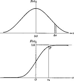
Consider an infinite set of values of v(tf) sampled over an infinite ensemble of the function. The amplitude distribution or probability density of this set is then expressed by the function f(v), Fig. 2.8a, defined such that the lim f{v) Av is the fraction of all the samples that fall in the range Av.

Av—>®

This fraction is then given by the area of the strip shown. It follows that

The cumulative distribution is given by

(2.6,24a)

and is illustrated in Fig. 2.86. The ordinate at P gives the fraction of all the samples that have values v < The distribution that we usually have to deal with in turbulence and noise is the normal or Gaussian distribution, given by

(2.6,25)

where a is the standard deviation or variance of v, and is exactly the rms value used in (2.6,8) = v (2.6,26)

Note that a can be computed from either the autocorrelation (2.6,7) or the spectrum function (2.6,11).

The correlation function (or covariance) of two functions vft) and vs(t) is defined as

Ліг(т) = <*>i (t)vz(t + t)) (2.6,5)

i. e. as the average (ensemble or time) of the product of the two variables with time separation r. If vft) = v^(t) it is called the autocorrelation, otherwise it is the cross-correlation. If r = 0 (2.6,5) reduces to

^ia(O) = (vi ®a)

and the autocorrelation to

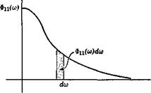
Fig. 2.7 Spectrum function.

Thus the area under the curve of the spectrum function gives the mean – square value of the random variable, and the area Ф(<у) dco gives the con­tribution of the elemental bandwidth dco (see Fig. 2.7).

In order to see the connection between the spectrum function and the harmonic analysis, consider the mean square of a function represented by a Fourier series, i. e.

V2(T) = — [Tvt)dt 2TJ-t

1 Гт / 00

^ — I 2 An cos nco0t + Bn sin nco0t 21 J—T n=o

00 •

A m cos mcOffi + Bm sin mco0t dt

m=0 /

Because of the orthogonality property of the trigonometric functions, all the integrals vanish except those containing A 2 and B2, so that

V* = 1№п + Bn2) (2.6,12)

72 = 0

From (2.3,126), A2 + B2 = 4 |Cy2, whence

— 00 00 00

»2 = 21 Cn2 = 2 l^nl2 = 2 C*nCn (2.6,13)

w=0 7i=—oo n=—oo

where the * denotes, as usual, the conjugate complex number.

The physical significance of Gn2 is clear. It is the contribution to v2 that comes from the spectral component having the frequency nco0. We may rewrite this contribution as

Now writing a>„ = bco and interpreting bv2 as the contribution from the hand width (n — J)co0 < a> < (n + h)OJo> we have

— n*rt

ЬУ = S-і bw

The summation of these contributions for all n is v2, and by comparison with (2.6,11) we may identify the spectral density as

G*C

Фи(а>) = lim n n

to0->0 ft>0

More generally, for the cross spectrum of and ;

G*C, *o ft>0

Now in many physical processes v2 can be identified with instantaneous power, as when v is the current in a resistive wire or the pressure in a plane acoustic wave. Generalizing from such examples, v2(t) is often called the instantaneous power, v2 the average power, and Фп(со) the power spectral density. By analogy Ф12(со) is often termed the cross-power spectral density.

From (2.6,9), and the symmetry properties of Il12 given by (2.6,86), and by noting that the real and imaginary parts of e~i<OT are also respectively even and odd in т it follows easily that

Фі2(о>) = Ф*і(<п) (2.6,17а)

The result given in (2.6,17) is sometimes expressed in terms of Fourier trans­forms of truncated functions as follows. Let v{(t; T) denote the truncated function

v((t;T) = vt(t) for 111 < T

v((t;T) =0 for Ы > T (2.6,18)

(2.6,19)

he the associated Fourier transform. Comparing (2.6,19) with (2.3,1) in Table 2.1 (w = nm0) we see that

С1п = ^У,(псо0;Т) Ztt

Фізм =lim V*(nco0; T) ■ V,(noJa; T)

U)n-*0 4:77

On substitution of co0 = tt/T and со = ncog, this becomes finally,

(2.6,22a)

CORRELATION AND SPECTRUM OF A SINUSOID

After integrating and taking the limit, the result is the cosine wave

R(t) = — cos Or
2

It follows that the spectrum function is 1/2-7Г times the Fourier transform of (2.6,23), which from Table 2.2 is

(2.6,23 a)

i. e. a pair of spikes at frequencies ±£2.

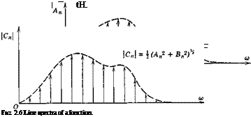
The deviation v(t) may be represented over the interval — T to T (fx having been set equal to zero) by the real Fourier series (2.3,12), or by its complex counterpart (2.3,2). Since v(t) has a zero mean, then from (2.3,12c) A0 — 0. Since (2.3,12cZ) shows that B0 also is zero, it follows from (2.3,126) that G0 = 0 too. The Fourier series representation consists of replacing the actual function over the specified interval by the sum of an infinite set of sine and cosine waves—i. e. we have a spectral representation of x(t). The amplitudes and frequencies of the individual components can be portrayed by a line spectrum, as in Fig. 2.6. The lines are uniformly spaced at the interval a)0 = 7т/T, the fundamental frequency corresponding to the interval 2T.

The function described by the Fourier series is periodic, with period 2 T, while the random function we wish to represent is not periodic. Nevertheless, a good approximation to it is obtained by taking a very large interval 2 T. This makes the interval co0 very small, and the spectrum lines become more densely packed.

If this procedure is carried to the limit T —* oo, the coefficients An, Bn, Gn all tend to zero, and this method of spectral representation of x(t) fails. This limiting process is just that which leads to the Fourier integral (see

2.3,4 to 2.3,6) with the limiting value of Gn leading to C(o>) as shown by (2.3,13). A random variable over the range — oo < t < oo does not satisfy the condition for G(w) to exist as a point function of со. Nevertheless, over any infinitesimal dw there is a well-defined average value, which allows a proper representation in the form of the Fourier-Stieltjes integral

v{t) = Г eiatdc (2.6,4)

J (0*=—00

It may be regarded simply as the limit of the sum (2.3,2) with исо0 —* со and Gn —>■ dc. Equation (2.6,4) states that we may conceive of the function

v(t) as being made up of an infinite sum of elementary spectral components, each of bandwidth dm, of the form eiwt, i. e. sinusoidal and of amplitude dc. If the derivative dcjdm existed, it would be the G(m) of (2.3,4).

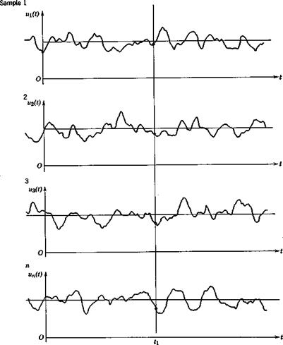
In the above discussion, the time average of a single function was used. Another important kind of average is the ensemble average. Imagine that the physical situation that produced the random variable of Fig. 2.4 has been repeated many times, so that a large number of records are available as in Fig. 2.5.

The ensemble average corresponding to the particular time is expressed in terms of the samples u^tj) as

<«(<i)> =lim (u(tv n)) =lim – [w1(i1) + м2(У ‘ ’ ’ (2.6,3)

n-* oo n-* oo 71

If the process is stationary, (ад(^)) — (и), independent of tv The process is said to be ergodic if the ensemble and time averages are the same, i. e. (и) = й. This will be the case, for example, if the records are obtained from a single physical system with random starting conditions. In this book we are con­cerned only with stationary ergodic processes.

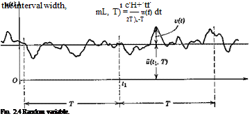
Consider a random variable u(t), as shown in Fig. 2.4. The average value of «(f) over the interval (tx — T) to (t1 + T) depends on the mid-time tv and

The function is said to have a stationary mean value й if the limit of «(fj, T) as T —*■ oo is independent of t±: i. e.

1 rti+T

it = lim — u(t) dt (2.6,2)

T^oo2Tjh-T

If, in addition, all other statistical properties of «(f) are independent of tv then it is a stationary random variable. We shall be concerned here only with such functions, and, moreover, only with the deviation v(t) from the mean (see Fig. 2.4). The average value of v(t) is zero.

There are important problems in flight dynamics that involve the response of systems to random inputs. Examples are the motion of an airplane in

atmospheric turbulence, aeroelastic buffeting of the tail when it is in the wing wake, and the response of an automatically controlled vehicle to random noise in the command signal. The method of describing these random functions is the heart of the engineering problem, and determines which features of the input and the response are singled out for attention. The treatment of such functions is the subject matter of generalized harmonic analysis. It is not our intention to present a rigorous treatment of this involved subject here. However, a few of the more important aspects are discussed, with emphasis on the physical interpretation.

When two or more of the roots are the same, then the expansion theorem given above fails. For then, after canceling one of the repeated factors from D(s) by the factor (s — aT) of the numerator, still another remains and becomes zero when s is set equal to ar. Some particular cases of equal roots are shown in Table 2.3, items 6, 7,11, and 12. The method of partial fractions, coupled with these entries in the table, suffices to deal conveniently with most cases encountered in stability and control work. However, for cases not conveniently handled in this way, a general formula is available for dealing with repeated roots. Equation (2.5,6) is used to find that part of the solution which corresponds to single roots. To this is added the solution corresponding to each multiple

THE USE OF TABLES OF TRANSFORMS

Extensive tables of transforms (like Table 2.3) have been published (see Bibliography) which are useful in carrying out the inverse process. When the transform involved can be found in the tables, the function x(t) is obtained directly.

THE METHOD OF PARTIAL FRACTIONS

In some cases it is convenient to expand the transform x(s) in partial fractions, so that the elements are all simple ones like those in Table 2.3. The function x(t) can then be obtained simply from the table. We shall demonstrate this procedure with an example. Let the second-order system of Sec. 2.4 be initially quiescent, i. e. x(0) = 0, and ж(0) = 0, and let it be acted upon by a constant unit force applied at time f = 0. Then /(f) = 1(f), and /(.s) = 1 js (see Table 2.3). From (2.4,4), we find that

ф2 + 2 £cons + con2)

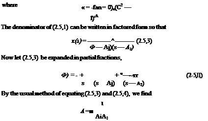
Let us assume that the system is aperiodic: i. e. that £ > 1. Then the roots of the characteristic equation are real and equal to

Z12 = n ± со’

Therefore

m = w. + m – + ід2(я2 – At) s s Ai s • A2 By comparing these three terms with items 3 and 8 of Table 2.3, we may write down the solution immediately as

x(t) = — H———————————– ——- e A±A2 A| (А і A2) A2(A, ■ A2) = J_ [l, n – e(n+a>’)t _ n + °> ‘еЫ-т’Н ton2 L 2w’ 2ft)’ .

(2.5,5)

HEAVISIDE EXPANSION THEOREM When the transform is a ratio of two polynomials in s, the method of partial fractions can be generalized. Let

where N(s) and D(s) are polynomials, and the degree of D(s) is higher than that of N(s). Let the roots of the characteristic equation D(s) = 0 be ar, so that

D(s) = (s – aq)(s – a2) ■ ■ ■ (s – an)

Then the inverse of the transform is

The effect of the factor (s — ar) in the numerator is to cancel out the same factor of the denominator. The substitution s = ar is then made in the reduced expression.

In applying this theorem to (2.5,3), we have the three roots al = 0, a2 = ^i> «з = ^21 and N(s) = 1. With these roots, (2.5,5) follows immediately from (2.5,6).

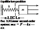
The Laplace transform finds one of its most important uses in the theory of linear differential equations. The commonest application in airplane dynamics is to ordinary equations with constant coefficients. The technique for the general case is given in Sec. 3.2. Here we illustrate it with the simple but important example of a spring-mass-damper system acted on by an external force (Fig. 2.3). The differential equation of the system is

* + 4<onx + co2x = f(t) (2.4,1)

2£(ои is the viscous resistance per unit mass, c/m, со,,2 is the spring rate per unit mass, kjm, and f(t) is the external force per unit mass. The Laplace

transform of (2.4,1) is formed by multiplying through by e~si and integrating term by term from zero to infinity. This gives

& И +

Upon using the results of Sec. 2.3, this equation may be written S2X + 2 lmnsx + 0Jn2x = / + x(0) + вж(0) + 2£conx(0)

or щв) = /+ *(0) + (« + 2Ccu>(0)

s2 + 2 t, a>ns + eon2

The original differential equation (2.4,1) has been converted by the trans­formation into the algebraic equation (2.4,3) which is easily solved (2.4,4) to find the transform of the unknown function. In the numerator of the right-hand side of (2.4,4) we find a term dependent on the excitation (/), and terms dependent on the initial conditions [i(0) and ж(0)]. The denomi­nator is the characteristic polynominal of the system. As exemplified here, finding the Laplace transform of the desired solution x(t) is usually a very simple process. The heart of the problem is the passage from the transform x(s) to the function x(t). Methods for carrying out the inverse transformation
are described in Sec. 2.6. Before proceeding to these, however, some general comments on the method are in order.

One of the advantages of solving differential equations by the Laplace transform is that the initial conditions are automatically taken into account. When the inverse transformation of (2.4,4) is carried out, the solution applies for the given forcing function f(t) and the given initial conditions. By contrast, when other methods are used, a general solution is usually obtained which has in it a number of arbitrary constants. These must sub­sequently be fitted to the initial conditions. This process, although simple in principle, becomes extremely tedious for systems of order higher than the third. A second convenience made possible by the transform method is that in systems of many degrees of freedom, represented by simultaneous differential equations, the solution for any one variable may be found independently of the others.

The transform of an integral can readily be found from that derived above for a derivative. Let the integral be

у — jx(t) dt

and let it be required to find y(s). By differentiating with respect to t, we get

г-*»

EXTREME VALUE THEOREMS

Equation (2.3,14) may be rewritten as

Л0О

—x(0) + sx(s) = I e~stx(t) dt rT

= lim e~stx(t) dt

T-* oo Jo

We now take the limit s —► 0 while T is held constant, i. e.

CT

= lim x(t) dt = lim x(T) — a;(0)] T-* oo Jo T-* 00

This result, known as the final value theorem, provides a ready means for determining the asymptotic value of x(t) for large times from the value of its Laplace transform.

In a similar way, by taking the limit s —*■ oo at constant T, the integral vanishes for all finite x(t) and we get the initial value theorem.

lim sx(s) = x(0)

S-¥ CO