Category Dynamics of Flight

Impulse Response

The system is specified to be initially quiescent and at time zero is subjected to a sin­gle impulsive input

eft) = 8(t) (7.3,1)

The Laplace transform of the ith component of the output is then

x,(s) = Gfs)8(s)

which, from Table (A. l), item 1, becomes

= Gifs)

This response to the unit impulse is called the impulse response or impulsive admit­tance and is denoted hft). It follows that

hfs) = G^s) (a)

that is, G(s) is the Laplace transform of h(t)

Gfs) = f hft)e”dt

•in

From the inversion theorem, (A.2,11) lift) is then given by

Kf t) = ^7 j[ G,/s)eH ds (7.3,3)

Now if the system is stable, all the eigenvalues, which are the poles of G„(.v) lie in the left half of the і plane, and this is the usual case of interest. The line integral of

(7.3,3) can then be taken on the imaginary axis, s = і to, so that (7.3,3) leads to

h,/t) = -1- f eiM%(ico) doj (7.3,4)

that is, it is the inverse Fourier transform of G, y(/a>). The significance of Си(іш) will be seen later.

For a first-order component of Fig. 7.4 with eigenvalue A the differential equa­tion is

x — Ax = c (7.3,5)

for which we easily get

. 1

G(s) = h(s) = ——— (7.3,6)

s — A

The inverse is found directly from item 8 of Table A. 1 as

h(t) = ex’

For convenience in interpretation, A is frequently written as A = — 1/Г, where T is termed the time constant of the system. Then

h(t) = e-^ (7.3,7)

A graph of h{t) is presented in Fig. 1.5a, and shows clearly the significance of the time constant T.

For a second-order component of Fig. 7.4 the differential equation is

У + Ч^пУ + = c

where x = [y yY is the state vector. It easily follows that

Let the eigenvalues be A = n± iu>, where

n =

to (Г2)"2

then h(s) becomes

1

(s — n — ia))(s — n + ico) 1

(s — n)2 + ш2

and the inverse is found from item 13, Table A. l to be

1

h(t) = — ent sin cot (7.3,11)

CO

For a stable system n is negative and (7.3,11) describes a damped sinusoid of fre­quency co. This is plotted for various £ in Fig. 7.6. Note that the coordinates are so chosen as to lead to a one-parameter family of curves. Actually the above result only applies for I < 1. The corresponding expression for £ > 1 is easily found by the same method and is

where

a,’ = con(£2 – 1 )1/2

Graphs of (7.3,12) are also included in Fig. 7.6, although in this case the second-or­der representation could be replaced by two first-order elements in series.

7.4 Step-Function Response

This is like the impulse response treated above except that the input is the unit step function I(t), with transform ls (Table A. l). The response in this case is called the step response or indicial admittance, and is denoted It follows then that

(a)

(7.4Д)

(b)

Since the initial values (at t = 0 ) of h^t) and Ml ^t) are both zero, the theorem (A.2,4) shows that

Thus siyit) can be found either by direct inversion of (7.4,lb) or by integration of hjft). By either method the results for first – and second-order systems are readily ob­tained, and are as follows (for a single input/response pair the subscript is dropped):

Second-order system:

For £ > 1, see Appendix A.2.

Graphs of the indicial responses are given in Figs. 7.5b and 7.7.

The asymptotic value of M(t) as t —> °° is called the static gain K. Applying the final value theorem (A.2,12) (7.4,1) yields

lim sd(t) = lim s. A(s) = lim G(s)

К = lim G(s)

s—*0

f—>oo s—>0 s—*0

Response of Linear/Invariant Systems

For linear/invariant systems there are four basic single-input, single-response cases, illustrated in Fig. 7.2. They are characterized by the inputs, which are, respectively:

1. a unit impulse at t = 0

2. a unit step at / = 0

3. a sinusoid of unit amplitude and frequency /

4. white noise

In the first two the system is specified to be quiescent for t < 0 and to be subjected to a control or disturbance input at t = 0. In the last two cases the input is presumed to have been present for a very long time. In these two the system is assumed to be sta­ble, so that any initial transients have died out. Thus in case 3 the response is also a steady sinusoid and in case 4 it is a statistically steady state. We discuss the first three of these cases in the following, but the fourth, involving the theory of random processes, is outside the scope of this text. The interested reader will find a full ac­count of that topic in Etkin, 1972.

0(s)

(4)

Figure 7.2 The four basic response problems. (1) Impulse response. (2) Step response. (3) Frequency response. (4) Response to white noise.

TRANSFER FUNCTIONS

A central and indispensable concept for response analysis is the transfer function that relates a particular input to a particular response. The transfer function, almost uni­versally denoted G(s), is the ratio of the Laplace transform of the response to that of the input for the special case when the system is quiescent for t < 0. A system with n state variables xt and m controls c, would therefore have a matrix of nm transfer func­tions Gfs).

The Laplace transform of (7.1,4) is.

sx — Ax – f – Be

(7.2,1)

hence

(si – A)x = Be

and

x = Gc

(a)

(7.2,2)

where

G(s) = (si – A) ‘B

(b)

is the matrix of transfer functions. The response of the ith state variable is then given by

Ф) = ^С, р)ф) (7.2,3)

j

For a single-input single-response system with transfer function G(s) we have simply

Systems in series.

SYSTEMS IN SERIES

When two systems are in series, so that the response of the first is the input to the second, as in Fig. 7.3, the overall transfer function is seen to be the product of the two. That is,

Xi(s) = Gfs)c(s)

and x2(s) = G2(s)xl(s) = G2(s)G,(s)c(s)

Thus the overall transfer function is

G(s) = x2(s)/c(s) = G,0)G20) (7.2,5)

Similarly for n systems in series the overall transfer function is

G(s) = G,(*)G2(s)-G„(s) (7.2,6)

HIGH-ORDER SYSTEMS

High-order linear/invariant systems, such as those that occur in aerospace practise, can always be represented by a chain of subsystems like (7.2,6). This is important, because the elemental building blocks that make up the chain are each of a simple kind—either first-order or second-order. To prove this we note from the definition of an inverse matrix (Appendix A. l) that

adj (si – A)

det (si — A)

We saw in Sec. 6.1 that det (A — si) is the characteristic polynomial of the system. We also have, from the definition of the adjoint matrix as the transpose of the matrix of cofactors, that each element of the numerator of the right side of (7.2,7) is also a polynomial in s. (See Exercise 7.1.) Thus it follows from (1.2,2b), on noting that В is a matrix of constants, that each element of G is a ratio of two polynomials, which can be written as

Np)

m

in which /(s) is the characteristic polynomial. It is seen that all the transfer functions of the system have the same denominator and differ from one another only in the dif­ferent numerators. Since f(s) has the roots A, . . . A,„ the denominator can be factored to give

,

" (s – A,)C? – A2) ••• (s – A„)

Figure 7.4 High-order systems as a “chain.”

Now some of the eigenvalues Ar are real, but others occur in complex pairs, so to ob­tain a product of factors containing only real numbers we rewrite the denominator thus

m 1/2 (n+m)

f(s)=r[(s-Ar) П (s2 + a^ + br) (7.2,10)

r= 1 r=m+ 1

Here Ar are the m real roots of f(s) and the quadratic factors with real coefficients a, and br produce the (n — m) complex roots. It is then clearly evident that the transfer function (7.2,9) is also the overall transfer function of the fictitious system made up of the series of elements shown in Fig. 7.4. The leading component Nfs) is of course particular to the system, but all the remaining ones are of one or other of two simple kinds. These two, first-order components and second-order components, may there­fore be regarded as the basic building blocks of linear/invariant systems. It is for this reason that it is important to understand their characteristics well—the properties of all higher-order systems can be inferred directly from those of these two basic ele­ments.

LATERAL CONTROL

The lateral controls (the aileron and rudder) on a conventional airplane have three principal functions.

1. To provide trim in the presence of asymmetric thrust associated with power plant failure.

2. To provide corrections for unwanted motions associated with atmospheric tur­bulence or other random events.

3. To provide for turning maneuvers—that is, rotation of the velocity vector in a horizontal plane.

The first two of these purposes are served by having the controls generate aero­dynamic moments about the x and z axes—rolling and yawing moments. For the third a force must be provided that has a component normal to V and in the horizontal plane. This is, of course, the component L sin ф of the lift when the airplane is banked at angle ф. Thus the lateral controls (principally the aileron) produce turns as a secondary result of controlling ф.

Ordinarily, the long-term responses to deflection of the aileron and rudder are very complicated, with all the lateral degrees of freedom being excited by each. Solu­tion of the complete nonlinear equations of motion is the only way to appreciate these fully. Certain useful approximations of lower order are however available.

THE CONTROL EQUATIONS

Whereas the study of stability that was the subject of Chap. 6 is generally sufficiently well served by the linear model of small disturbances from a condition of steady flight, the response of an airplane to control action or configuration change can in­volve very large changes in some important variables, especially bank angle, pitch angle, load factor, speed, and roll rate. Consequently nonlinear effects may be present in any of the gravity, inertia, and aerodynamic terms. An accurate system model ca­pable of dealing with these large responses must therefore begin with the more exact equations (4.7,1)—(4.7,4). These would normally be reorganized into first-order state space form for subsequent integration by a Runge-Kutta or other integration scheme. Equations (4.7,3d-f) and (4.7,4) are already in the required form. However (4.7,1) and (4.7,2) need to be rearranged. In particular, (4.7,2a and c) need to be solved si­multaneously for p and r. The functional form that results is as follows:

X

tiE = f(vE, wE, q, г в, X’) + —

m

vE = f(uE, wE, p, г, в, Ф, Y’) H– 1

m

wE = f(uE, vE, p, q, 0, </>, Z’) + —

m

P = f(p, g, r, L’, N’) + -f + 4iVc

^ X

Mc

q = ftp, r, M’) + — ly

r = f{p, q,r, L’,N’) + ^ +rj, c

o = fig, Г, Ф)

Ф = fiP> g, г, в, Ф)

In the preceding equations, the subscript c denotes the control forces and moments, and the prime on force and moment symbols denotes the remainder of the aerody­namic forces and moments. The solution of these equations would require that an aerodynamic submodel be constructed for each case to calculate the forces and mo­ments at each computing step from a knowledge of the state vector, the control vec­tor, the current configuration, and the wind field. To follow this course in extenso would take us beyond the scope of this text, so for the most part the treatments that follow are restricted to the responses of linear invariant systems, that is, ones de­scribed by (4.9,20) with A and В constant viz

x = Ax + Be (7.1,4)

Although we are thereby restricted to relatively small departures from the steady state, these responses are nevertheless extremely useful and informative. Not only do they reveal important dynamic features, but when used in the design and analysis of automatic flight control systems that are designed to maintain small disturbances they are in fact quite appropriate.

Table 7.1

Dimensional Control Derivatives

X

z

M

Se

C^puls

CzSiPulS

C„shpulSc

Cxsipu20S

Czai? PuoS

Qng 2pU0Sc

°n

Y

L

N

8*

Cyshpu20S

clshpu20Sb

C„spu20Sb

8r

CyahpuoS

C, spu20Sb

C„shpu20Sb

In the examples that follow, we use {8e, S;,j for the longitudinal controls, elevator and throttle; and {5a, S,} for the lateral controls, aileron, and rudder. The aerody­namic forces and moments are expressed just like the stability derivatives in terms of sets of nondimensional and dimensional derivatives. The nondimensional set is the partial derivatives of the six force and moment coefficients {Cx, Cy, Cz, Ch Cm, C„} with respect to the above control variables, such as C = c)CJ<)8e or C,^ = dCJd8a, and so on. The dimensional derivatives are displayed in Table 7.1.

The powerful and well-developed methods of modem control theory are directly applicable to this restricted class of airplane control responses. Before proceeding to specific applications, however, we first present a review of some of the highlights of the general theory. Readers who are well versed in this material may skip directly to Sec. 7.6.

Response to Actuation of the. Controls-Open Loop

7.1 General Remarks

In this chapter we study how an airplane responds to actuation of the primary con­trols—elevator, aileron/spoiler, rudder, and throttle. These are of course not the only controls that can be incorporated in the design of an airplane. Also used, less fre­quently, are vectored thrust and direct lift control. Closely related to the control-re­sponse problem is the response of the airplane to an in-flight change of configuration such as flap deflection, lowering the undercarriage, releasing stores or armaments, deploying dive brakes, or changing wing sweep. The analysis of the response of the airplane to any of these uses methods generally similar to those that are described in the following. In the remainder of this chapter, it is assumed that there is no wind.

LONGITUDINAL CONTROL

The two principal quantities that need to be controlled in symmetric flight are the speed and the flight-path angle, that is to say, the vehicle’s velocity vector. To achieve this obviously entails the ability to apply control forces both parallel and perpendicu­lar to the flight path. The former is provided by thrust or drag control, and the latter by lift control via elevator deflection or wing flaps. It is evident from simple physical reasoning (or from the equations of motion) that the main initial response to opening the throttle (increasing the thrust) is a forward acceleration, i. e. control of speed. The main initial response to elevator deflection is a rotation in pitch, with subsequent change in angle of attack and lift, and hence a rate of change of flight-path direction. When the transients that follow such control actions have ultimately died away, the new steady state that results can be found in the conventional way used in perfor­mance analysis. Figure 7.1 shows the basic relations. The steady speed V at which the airplane flies is governed by the lift coefficient, which is in turn fixed by the elevator angle—see Fig. 2.19. Hence a constant Se implies a fixed V. The flight-path angle у = в – ax at any given speed is determined, as shown in Fig. 7.1, by the thrust. Thus the ultimate result of moving the throttle at fixed elevator angle (when the thrust line passes through the CG) is a change in у without change in speed. But we saw above that the initial response to throttle is a change in speed—hence the short-term and long-term effects of this control are quite contrary. Likewise we saw that the main initial effect of moving the elevator is to rotate the vehicle and influence y, whereas the ultimate effect at fixed throttle is to change both speed and y. The short­term and long-term effects of elevator motion are therefore also quite different. The

total picture of longitudinal control is clearly far from simple, and the transients that connect the initial and final responses require investigation. We shall see in the fol­lowing that these are dominated by the long-period, lightly damped phugoid oscilla­tion, and that the final steady state with step inputs is reached only after a long time. These matters are explored more fully in the following sections.

Effects of Wind

In all the preceding examples, the atmosphere has been assumed to be at rest or to have a velocity uniform in space and constant in time. Since this is the exceptional rather than the usual case, it is necessary to examine the effects of nonuniform and unsteady motion of the atmosphere on the behavior of flight vehicles. The principal effects are those associated with atmospheric turbulence, and these are treated at some length in Etkin (1972, 1981). However, quite apart from turbulence, the wind
may have a mean structure which is not uniform in space, that is, there can be spatial gradients in the time-averaged velocity. The examples of most concern are down – bursts and the boundary layer next to the ground produced by the wind blowing over it. Downbursts are vertical outflows from low level clouds that impinge on the ground, somewhat in the manner of a circular jet, and spread horizontally. The result­ing wind field has strong gradients, both horizontal and vertical. A number of air­plane accidents have been attributed to this phenomenon.

In order to introduce wind into the analytical model, we must make any alter­ations that may be needed, because of the presence of the wind, to the aerodynamic forces and moments. In the trivial case when the wind is uniform and steady, no change is necessary to the representation of aerodynamic forces from that used be­fore. However, turbulence and wind gradients may require such changes.

Since the linear model that was developed in Chap. 4 is based on small distur­bances from a steady reference condition, and since there is no such steady state when the aircraft is landing or taking off through a boundary layer or downburst, the linear model is of limited use in these situations. For this kind of analysis, one must use the nonlinear equations (4.7,1)—(4.7,5) and introduce a model for the aerody­namic forces that embraces the whole range of speeds and attitudes that will occur throughout the transient (Etkin, B. and Etkin, D. A. (1990)). Such an analysis is be­yond the scope of this volume.

There is one relevant steady state, however, that can be investigated with the lin­ear model, and that is horizontal flight in the boundary layer. The planetary boundary layer has characteristics quite similar to the classical flat-plate turbulent boundary layer of aerodynamics. The vertical extent of this layer in strong winds depends mainly on the roughness of the underlying terrain, but is usually many hundreds of feet. Figure 6.17 shows the power-law profiles associated with different roughnesses. These are all of the form

W = khn

where, as indicated in the figure, h is height above the ground. The vertical gradient is then given by

For example, for smooth terrain (n = 0.16), and for a wind of 50 fps at 50 ft altitude, the gradient would be dW/dh = 0.16 fps/ft.

By way of example, we shall analyze what effect the vertical wind gradient has on the longitudinal modes of the STOL airplane of Sec. 6.6 in low speed flight, when wind effects can be expected to be largest. In order to generate the analytical model, we go back to the exact equations (4.7,1) et seq. The longitudinal equations, when linearized for small perturbations around a reference state of horizontal flight at speed u0 and в0 = 0 are

AX — mgQ = mAiib A Z = m(w’ — uEq) AM = Iyq 6=q

ZE = – иЬв + WE

A, feet

Figure 6.17 Profiles of mean wind velocity over level terrains of differing roughness. (After A. G. Davenport, 1960)

The wind is specified to vary linearly with altitude with gradient Г = dW/dzE and to be parallel to the хг plane. The wind vector is prescribed in frame FE as

We will assume that this implies a tailwind of strength W0 at the reference height. For a wind that increases with altitude, Г = —sgn(W0)|r|. To convert WE to body axes, we use the transformation matrix L/JE [the transpose of (4.4,3)] for small angles and ф = ф = 0 to get (see Exercise 6.6)

" W0 + rzE "

” W0 + TzE

WB =

0

as

0

(W0 + TzE)e

w0e

In the third component of (6.9,5) we have neglected the second-order product zE6. We can now use (6.9,5) together with Vе = V + W to eliminate uE and wE from

(6.9,3) with the result

AX — mgO = m( Ай + TzF)

A Z = m(w + W06 — uEq)

AM = Iyq (6.9,6)

в=Ч

zE = ~ueQ + w + W06

We note that uE = u0 + W0 and eliminate 6 and zE from the right side of (6.9,6) with the result

AX — mg6 = т(Ай + Г[—и0в + w])

A Z = m(w — u0q)

AM = I# (6.9,7)

6=q

ZE = UqO + w

It is observed that the only explicit effect of wind on the system equations in this case is the term containing Г on the right side of the first equation. Since a uniform wind (i. e., Г = 0) does not affect the airplane dynamics the system must be indepen­dent of W0, and we see that W() does indeed not appear anywhere in the equations. In addition to what we see in (6.9,7), however, there are some implicit effects of the wind gradient on the aerodynamic derivatives.

It is clear that the changes in pressure distribution over the surfaces of a vehicle, and hence its basic aerodynamic derivatives, are not the same when the incident flow has a gradient Г as when it is spatially uniform. Two simple examples suffice to make this clear. (1) When there is a perturbation Да from the reference state, the tail moves downward into a region of lower air velocity and on this account one would expect CmJ to be smaller than normal. (2) When the wing rolls through an angle ф, the right tip moves into a low-wind region, and the left tip into a high-wind region. The gradi­ent in velocity across the span is like that associated with yaw rate r, and hence we should expect values of С1ф and СПф proportional to the wing contributions to Clr and

C„r. Note that for upwind flight this leads to an unstable roll “stiffness” С! ф > 0 where none existed before (Ct is negative for downwind flight).

Reasonable estimates of the major changes in the basic derivatives associated with Г can be made from available aerodynamic theories, but a complete account of these is not currently available, and to develop them here would take us too far afield. Instead we simply incorporate the additional terms given by (6.9,7) into the longitu­dinal equations of motion and note the extent of the changes they make in the charac­teristic modes previously calculated. The appropriate matrix for this case is obtained from (4.9,18) by adding the two terms containing Г, and is given by (6.9,8).

(6.9,8)

In (6.9,8), A’ is the З X 4 matrix consisting of the last three rows of the matrix of

(4.9,18) , with 0O = 0.

An example of the results for the STOL airplane is shown in Figs. 6.18 and 6.19. The numerical data used was the same as in Sec. 6.6, with wind gradient variable from -0.30 fps/ft (the headwind case) to +0.30 fps/ft (the tailwind case). The effects on both the phugoid and pitching modes are seen to be large. A strong headwind de­creases both the frequency and damping of the phugoid, and a strong tailwind changes the real pair of pitching roots into a complex pair representing a pitching os­cillation of long period and heavy damping.

-0.5

-1.0

Figure 6.19 Effect of wind gradient on short-period roots—STOL airplane. Cw = 4.0.

DUTCH ROLL MODE

A physical model that gives an approximation to the lateral oscillation is a “flat” yawing/sideslipping motion in which rolling is suppressed. The corresponding equa­tions are obtained from (4.9,19) by setting p = ф = 0 and dropping the second (rolling moment) equation. The term in Yr is also neglected in the first equation. The
result is

V = fyvV — u0r r = Nvv + Nrr

The corresponding characteristic equation is readily found to be

A2 – (% + Mr)A + ($ljrr + u0Nv) = 0 (6.8,12)

The result obtained from (6.8,12) for our example is XnR = —0.1008 ± 0.9157г, or

T = 6.86 sec

AU= 1.0

The approximation for the period is seen to be useful (an error of about 3%) but the damping is very much overestimated.

There is another approximation available for the damping in this mode that may give a better answer. It follows from the fact that the coefficient of the next-to-highest power of A in the characteristic equation is the “sum of the dampings” (see Exercise 6.4). Thus it follows from the complete system matrix of (6.8,2) that

2 nDR + R + s = e9v + ^£p + Яг

or nDR = U°!)v + £p + Mr-(AR + A5)} (6.8,13)

But the approximation (6.8,11) for the roll and spiral modes gives precisely

_ D

On using (6.8,11) we get the expression

Подпись: (6.8,14)l S

+ Nr + — Iff———-

К Щ

which is to be compared with + Яг) given by (6.8,12). The damping obtained from (6.8,14) is nDR = —0.0159, better than that obtained from (6.8,12) but still quite far from the true value of —0.0330. The simple average of the two preceeding ap­proximations for the Dutch Roll damping has also been used. In this instance it gives nDR = —0.0584, which although better is still 77% off the true value.

This example of an attempt to get an approximation to the Dutch Roll damping illustrates the difficulty of doing so. Although the approximation tends to be better at low values of CL, nevertheless it is clear that it must be used with caution, and that only the full system matrix can be relied on to give the correct answer.

ROLLING MODE

It was observed in Sec. 6.7 that the rolling convergence is a motion of almost a single degree of freedom, rotation about the x-axis. This suggests that it can be approxi­mated with the equation obtained from (4.9,19) by putting v = r = 0, and consider­ing only the second row, that is,

p = $„P (6-8,7)

which gives the approximate eigenvalue

XR = %P = LpH’x + I’zxNp (6.8,8)

The result obtained from (6.8,8) for the B747 example is AR = —0.434, 23% smaller than the true value -0.562. This approximation is quite rough.

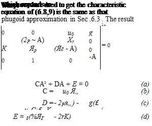
An alternative approximation has been given by McRuer et al. (1973). This ap­proximation leads to a second-order system, the two roots of which are approxima­tions to the roll and spiral modes. In some cases the roots may be complex, corre­sponding to a “lateral phugoid”—a long-period lateral oscillation. The approximation corresponds to the physical assumption that the side-force due to gravity produces the same yaw rate r that would exist with /3 = 0. Additionally Yp and Yr are ne­glected. With no approximation to the rolling and yawing moment equations the sys­tem that results for horizontal flight is

0 = ~u0r + g(f) (a)

p = !£vv + !£pp + £rr (b)

r = Jfvv + Ярр + Ягг (c) (6.8,9)

ROLLING MODE ROLLING MODE

Ф = P (d)

The result of applying (6.8,11) to the B747 example is

A, = -0.00734 and A* = -0.597

These are within about 1 % and 6% of the true values, respectively, so this is seen to be a good approximation for both modes, certainly much better than (6.8,7) for the rolling mode.

Approximate Equations for the Lateral Modes

As with the longitudinal modes we should like if possible to have useful analytical approximations to the lateral characteristics. We find that there are reasonable ap­proximations to all three modes, but the application of all such approximations must be made with caution. Their accuracy can really be verified only a posteriori, by comparison with exact solutions. They can only be used with confidence in situations similar to those in which they have previously been found to work well.

SPIRAL MODE

Comparison of the eigenvalues in Sec. 6.7 shows that Л for the spiral mode is two or­ders of magnitude smaller than the next larger one. This suggests that a good approx­imation to this root may be obtained by keeping only the two lowest-order terms in the characteristic equation, that is,

£>A + £ = 0 (6.8,1)

or Av = —E/D

where As denotes the real root for the spiral mode. Before deriving expressions for D and E, we rewrite the matrix of (4.9,19) in a more compact notation for convenience, including the approximation Yp = 0.

%

0

%

g cos 0O

A =

£v

£r

0

К

к

К

0

_ 0

1

tan 0O

0

The meanings of the symbols in (6.8,2) are obtained by comparison with (4.9,19), for example

Approximate Equations for the Lateral Modes Подпись: К h

and in the special case when the stability axes are also principal axes, I„ = 0 and

With the notation of (6.8,2), expanding det (A — ЛІ) yields

E = g[(£vNr – £rKv) cos 0O + (£рХи – £vMp) sin 0O] (a)

D = ~g(£v cos 0O + Jfv sin 0O) + °Hv(£rMp – £pKr) (6.8,3)

+ Щ<£^0 – £VMP) (b)

When the orders of the various terms in D are compared, it is found that the second term can be neglected entirely and YT can be neglected in rj>£. The approximation that then results is

D = ~g(£„ cos 0O + Mv sin 0O) + u0(£vXp – £pMv) (6.8,4)

The result obtained from (6.8,1), (6.8,3a), and (6.8,4) for the jet transport example of Sec. 6.7 is As. = —0.00725, less than 1% different from the correct value. Equation

(6.8,1) is seen to give a good approximation in this case.

It will be recalled that the coefficient E has special significance with respect to static stability (see Sec. 6.1). We note here that in consequence of (6.8,1) the spiral mode may exhibit exponential growth, and that the criterion for static lateral stability is

(£vMr – £rXv) cos 0O + (£PMV – £v. Kp) sin 0O > 0 (6.8,5)

On substituting the expanded expressions for £v and so forth, (6.8,5) reduces to

{Cifnr – C, Cn/1) cos 00 + (ClpCnfi – chcn) sin 00 > 0 (6.8,6)

Since some of the derivatives in (6.8,6) depend on CLo, the static stability will vary with flight speed. It is not at all unusual for the spiral mode to be unstable over some portion of the flight envelope (see Table 6.10 and Exercise 6.3).

EFFECT OF SPEED AND ALTITUDE

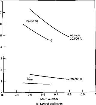
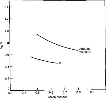
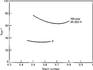
Even for the “basic” case of a rigid airplane at low Mach number, the variation of the lateral modes with speed and altitude may not be simple. This is because some of the lateral stability derivatives are dependent on the lift coefficient in complex ways. That is especially true of airplanes with swept wings and low aspect ratio for which Clfj in­creases markedly with CL. These effects will appear most strongly at low speed and high altitude, both of which require high CL. (Note that in the B747 example at M =

0. 8 and 40,000 ft, CL = 0.654, which is quite large for cruising flight.) For a rigid swept-wing airplane at low Mach number the period of the Dutch Roll mode would be expected first to increase and then to decrease as the airplane speed increases. The damping of this mode would be expected to be weak at low speed and to increase at higher speeds. The rolling convergence is well damped at all speeds, but the damping would normally increase with speed. The spiral mode is frequently unstable over some portion of the speed/altitude flight envelope, depending on the interplay of the derivatives that appear in (6.8,6). The characteristic times of this mode are, however, usually so long that the instability does not degrade the handling qualities unduly.

The effect of increasing altitude at fixed CL is primarily an increase in the damp­ing time constants of all the modes. The period of the Dutch Roll is not much af­fected.

When substantial aeroelastic and compressibility effects are added to the already complex behavior of the lateral modes, the result is an even more irregular pattern of modal characteristics. The data of (Heffley and Jewel, 1972) for the B747, repro­duced in Table 6.10 show this. (Note that a negative fh. l!f implies an unstable mode.) At the two lower altitudes, with relatively low values of CL, the modes are seen to be­have in a fairly regular way (see Fig. 6.16). However, at 40,000 ft and high Mach

Table 6.10

Variation of Lateral Modes with Speed and Altitude

Spiral

mode

Rolling

convergence

Lateral oscillation (Dutch Roll)

Altitude.

Mach

thctlf

half

Period

^half

ft

No.

(s)

(S)

(s)

(cycles)

0

0.45

35.7

0.56

5.98

0.87

0

0.65

34.1

0.44

4.54

0.71

20,000

0.5

76.7

0.93

7.3

1.58

20,000

0.65

64.2

0.76

5.89

1.33

20,000

0.8

67.3

0.85

4.82

1.12

40,000

0.7

-296

1.5

7.99

1.93

40,000

0.8

94.9

1.23

6.64

3.15

40,000

0.9

-89.2

1.45

6.19

1.18

EFFECT OF SPEED AND ALTITUDE

EFFECT OF SPEED AND ALTITUDE

(b) Rolling convergence

Figure 6.16 Variation of lateral modes with speed and altitude, (a) Lateral oscillation, (b) Rolling convergence, (c) Spiral mode.

EFFECT OF SPEED AND ALTITUDE

(c) Spiral mode

Figure 6.16 (Continued)

number the lateral behavior is quite irregular, especially the variation of the damping of all the modes with M. The spiral mode is seen to be unstable (albeit with long time constant) at both M = 0.7 and 0.9 but stable at M = 0.8. This behavior is primarily the result of the complex variation of C, with CL and M in this region.

Lateral Modes of a Jet Transport

We use the same airplane and flight condition as for the longitudinal modes in Sec.

6.2, and calculate the lateral modes. The nondimensional and dimensional derivatives are given in Tables 6.6 and 6.7. Using these, the system matrix of (4.9,19) is found to be (note that the state vector is [v p г фт.):

-0.0558

0

-774

32.2

-0.003865

-0.4342

0.4136

0

0.001086

-0.006112

-0.1458

0

0

1

0

0

This yields the characteristic equation

A4 + 0.6358Л3 + 0.9388Л2 + 0.5114Л + 0.003682 = 0 (6.7,2)

The stability criteria are

E = 0.003682 > 0 R = 0.04223 > 0

Lateral Modes of a Jet Transport

so there are no unstable modes.

Table 6.7

Dimensional Derivatives—B747 Airplane

Y(lb)

Lift-lb)

N(fi-lb)

u(ft/s)

-1.103 X 10³

-6.885 X 10⁴

4.790 X 10⁴

p(rad/s)

0

-7.934 X 10⁶

-9.809 X 10⁵

r(rad/s)

0

7.321 X 10⁶

-6.590 X 10⁶

Y(N)

Цт-N)

N(m-N)

u(m/s)

-1.610 X 10⁴

-3.062 X 10⁵

2.131 X 10⁵

p(rad/s)

0

-1.076 X 10⁷

-1.330 X 10⁶

r(rad/s)

0

9.925 X 10⁶

-8.934 x 10⁶

EIGENVALUES

The roots of (6.7,2) are

Mode 1 (Spiral mode): A, = -0.0072973

Mode 2 (Rolling convergence): A2 = -0.56248

Mode 3 (Lateral oscillation or Dutch Roll): A3 4 = —0.033011 ± 0.94655/

Table 6.8 shows the characteristic times of these modes. We see that two of them are convergences, one very rapid, one very slow, and that one is a lightly damped oscilla­tion with a period similar to that of the longitudinal short-period mode.

EIGENVECTORS

The eigenvectors corresponding to the above eigenvalues are given in Table 6.9. In addition to the basic 4 state variables, Table 6.9 contains two extra rows that show the values of the two state variables ф and yE (see Exercise 6.2).

MODE 1: THE SPIRAL MODE

From Table 6.9, we find the ratios of the angle variables in the spiral mode to be

р:ф:ф= -0.00119:—0.177:1

so that the motion is seen to consist mainly of yawing at nearly zero sideslip with some rolling. This is, of course, the condition for a truly banked turn, and this mode

Table 6.8

Characteristic Times—Lateral Modes

Mode

Name

Period (s)

th alf(S)

N half (cycles)

1

Spiral

95

2

Rolling

convergence

1.23

3

Lateral oscillation (Dutch Roll)

6.64

21

3.16

Table 6.9

Eigenvectors (polar form)

Spiral

Rolling convergence

Dutch Roll

Magnitude

Phase

Magnitude

Phase

Magnitude

Phase

P = 0

0.00119

OO

о

о

0.0198

180°

0.33

-28.Г

p

1.63 X 10~4

0.0712

0

О

OO

0.12

92.0°

r

9.20 X 10~4

180°

0.0040

0.037

-112.3°

Ф

0.177

OO

О

о

1.0

1.0

Ф

1.0

0.0562

180°

0.31

155.7°

Уе

uut*

7.772 X 10³

180°

7.65

1.69

-165.8°

can be thought of as a variable-radius turn. The aerodynamically important variables are

/3 :p:r = 1:—0.137:0.773

and the largest of these, /3, has already been seen to be negligibly small for moderate values of ф and ф. The aerodynamic forces in this mode are therefore very small, and it may be termed a “weak” mode. This is consistent with its long time constant.

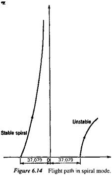
The flight path in the spiral mode can readily be constructed for any given initial yaw angle from the eigenvector. For example, with an initial ф of 20° (0.35 rad), we have from Table 6.9

ф = 0.35eAl’

v = 774(—0.00119)0.35eAl’ fps where A, = -0.0072973 s"1

From (4.9,19) and the above it follows that (for в0 = 0)

yE = —37079e-00072973′ ft xE = 774 t ft

Figure 6.14 shows the path—it is seen to be a long, smooth return to the reference flight path, corresponding to yE = 0. When the spiral mode is unstable as is fre­quently the case, ф, ф, and yE are all of the same sign, and of course all increase with time instead of decreasing, as shown in the figure.

MODE 2: THE ROLLING CONVERGENCE

The ratios of the angle variables in this mode are, from Table 6.9,

/З :ф:ф= -0.0198:1:-0.0562

The mode is evidently one of almost pure rotation around the x axis, and hence its name. The variables that are significant for aerodynamic forces are (/3, p, r) and they are in the ratios

/3 :p:r = 0.278:1:—0.0561

Подпись: *E

so that the largest rolling moment in this mode of motion is Clpp, and the r contribu­tions are negligible by comparison.

MODE 3: THE LATERAL OSCILLATION (DUTCH ROLL)

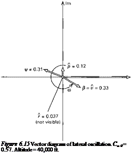
Подпись: Figure 6.15 Vector diagram of lateral oscillation. C„0 = 0.57. Altitude = 40,000 ft.

The vector diagram for this mode is shown in Fig. 6.15. It is seen that the three angle variables /3, ф, ф are of the same order of magnitude, that r is an order smaller, and

that /3 and ф are almost equal and opposite. It follows from (4.9,19) that yE is nearly zero. In dimensional terms, when ф = 20°, yF = 8 ft, whereas the wavelength of the oscillation is about 5000 ft. The vehicle mass center is seen to follow a nearly rectilinear path in this mode, the motion consisting mainly of yawing and rolling, the latter lagging the former by about 160° in phase.