Category FLIGHT MECHANICS MODELING and ANALYSIS

The nonlinear coupled 6DOF EOMs can be linearized using the small disturbance theory [2]. In using this theory, we assume that the excursions about the reference flight condition are small. Thus, we assume small values of the variables u, v, w, p, q, r, f, U. This theory cannot be applied to situations with large change in motion variables. In this approach, all the variables in the 6DOF model are expressed as a sum of a reference value (steady-state value) and a small perturbation, e. g.,

U = u0 + u V = v0 + v W = w0 + w

P = P0 + p Q = q0 + q R = r0 + r

The nonlinear translational accelerations from the full set of 6DOF equations (Equation 3.24) are expressed as

U = —qw + rv — g sin U + ax

V = —ru + pw + g cos U sin f + ay (5.2)

W = —pv + qu + g cos U cos f + az

From Equations 5.1 and 5.2, the u equation can be expressed in terms of perturbed variables as follows:

u = -(q + q0)(w + w0) + (r + r0)(v + v0) — g sin (U + 00) + (ax + ax0) (5.3)

Equation 5.3 can be simplified by neglecting products of the perturbations and using small-angle approximation. Also, assuming wings-level, symmetric reference flight, we have

w0 = v0 = p0 = q0 = r0 = f 0 = C0 = 0

Setting all disturbances in the perturbed U, V, W equations to zero gives the reference flight conditions as

axo = q0w0 — r0v0 + g sin 60

ay0 = r0 щ — p0w0 — g cos U0 sin f 0 (5.4)

aZ0 = p0v0 — q0u0 — g cos &0 cos f 0

U = — gU cos Uo + ax

v = —ru0 + gf cos U0 + ay w = +qu0 — gU sin U0 + az

The linearized implementation in Equation 5.5 is frequently used for

1. Routine batch analysis of large amount of data in cruise flight regimes

2. Analysis of small amplitude maneuvers

3. Where computational efficiency is important and nonlinear effects are minimal

Some of the simplification techniques used to get workable models for flight data analysis are (1) choice of coordinate systems, (2) linearization of model equations, (3) simplification using measured data, (4) use of decoupled models, (5) neglecting small terms, and (6) restricting excursions during maneuvers to permit the use of simplified models. Some of these simplification techniques are briefly discussed here.

5.2.1 Choice of Coordinate Systems

The selection of appropriate coordinate systems for EOMs plays an important role in simplification of EOM. The following are some of the important points to be considered [1]: (1) Body axis system is most suitable for defining rotational degrees of freedom. It is a normal practice to include the angular rates and the Euler angles in the aircraft state model, and the equations in body axis, under certain assumptions, can be considerably simplified; (2) Either of the polar or rectangular coordinate systems can be used for translational degrees of freedom; and (3) The polar axis system uses the (a, b, V) form, which involves wind axis coefficients CL and CD.

The wind axis coefficients introduce nonlinearities because of the way they are related to the body-axis force coefficients CX, CY, and CZ. However, a, b, and V are commonly measured quantities, which encourages the use of a polar coordinate system. The expressions for a, b, and V in observation equations are simple if polar coordinates are used for data analysis.

Linear accelerations are normally defined in terms of CX, CY, CZ, which suggests the use of u, v, w form of state equations. This form is particularly useful in the case of rotorcraft where the (a, b, V) form may lead to singularities. With the differential equations for u, v, w in the state model, the (a, b, V) expressions in the observation model will be nonlinear.

5.1 INTRODUCTION

Although simulation of nonlinear flight dynamics, in general, requires full six – degrees-of-freedom (6DOF) equations of motion (EOMs), it is not always necessary to use very complex and coupled models in the design of flight control laws, dynamic analysis, and handling qualities analysis procedures. Simple models with essential derivatives that capture the basic characteristics of the vehicle normally yield adequate results. However, caution must be exercised in simplifying the model too much as this may not be able to represent the system dynamics properly. Some of the reasons why flight analysts prefer simplified models are (1) full complex models are difficult to interpret and analyze, (2) it is possible to separate the model equations into independent subsets without much loss of accuracy, (3) ease of linearization, (4) unnecessary details that have little effect on system dynamics are avoided, (5) excursions during flight test maneuvers can be restricted to apply the assumption of linearity, and (6) easy to implement software codes are available for handling qualities analysis and parameter estimation. The simplification of nonlinear EOMs into workable and easily usable linear models can bring about connections between various aircraft configurations via the transfer-function (TF) analysis and frequency responses. The aircraft may be of different sizes and wing-body config­urations, but the dynamic characteristics may be the same. The TF analysis and zeros/poles disposition can be useful in assessing the dynamic characteristics of these aircraft, rotorcraft, missiles, UAVs (unmanned/uninhibited aerial vehicles), MAVs (micro-air vehicles), and airships. Simplified models are used in the design of autopilot control laws and in evaluation of handling qualities of the vehicle. The detailed effects of particular derivatives can be observed. Also, it becomes easy to obtain the aerodynamic derivatives of the vehicle from the flight data, using linear mathematical models in a parameter-estimation algorithm.

The TF analysis of the aircraft mathematical models gives a deeper insight into the effect of aircraft configurations on its dynamics. Aircraft configuration refers to the external shape of the aircraft and is related to the use of stores, center of gravity (CG) movement (aft, mid, and fore), flap settings, autopilot on or off condition, slat effect, airbrake deployment, etc. Aircraft dynamics for a particular configuration, at a
particular flight condition, are characterized by stability derivatives (Chapter 4). Understanding flight mechanics models via TF helps to properly interpret the effects of the configuration on flight responses as well as on aerodynamic derivatives.

The coupled nonlinear 6DOF EOMs discussed in Chapter 3 include nonlinea­rities because of the gravitational and rotation-related terms in the force equations and the appearance of products of angular rates in the moment equations. The dynamic pressure q also contributes to nonlinearity because it varies with the square of the velocity (q = 1 pV2). Apart from the nonlinearities contributed by the kin­ematic terms, the aerodynamic coefficients Cx, Cy, Cz, Q, Cm, and Cn may contain additional nonlinearities; for example, the lift coefficient due to horizontal tail, when expressed in Taylor’s series, may have the following form:

CLaH aH + CL8ede + CLS3 d3 + CLseaH deaH

The above model form may be useful in explaining nonlinearities arising from control surface deflections and flow effects at higher angles of attack. Analysis of a nonlinear model would generally require implementation of nonlinear programs. However, it would be worthwhile to determine simplified models that can be used in flight regimes where nonlinear effects are not important. In this chapter, we look at the various strategies adopted to simplify aircraft EOMs to obtain model forms that have practical utility and computation efficiency.

As we have seen earlier, aerodynamic forces and moments are numerically expressed in a Taylor’s series expansion of the instantaneous numerical values of the aircraft variables. Specifically, the aerodynamic forces and moments (in fact the aerody­namic coefficients) can be expressed as functions of Mach number M, engine thrust FT, and other aircraft motion and control variables a, b, p, q, r, f, U, 8e, 8a, and 8r. A complete set of aerodynamic coefficients can be represented as [11]

The forces acting on an aircraft are also expressed in terms of lift and drag: the lift force acts normal to the velocity vector V, and the drag force acts in the direction opposite to V. The nondimensional coefficients of lift and drag are denoted by CL and CD. Due to disposition of forces in x and z directions, it is required to resolve the relevant coefficients in the following way (see Exercise 4.4):

Cx = CL sin a — CD cos a Cz = — (CL cos a + CD sin a)

Here, the effect of AOSS is neglected. If AOA is small we can further simplify these equations as

Cx = Cia — Cd Cz = —(Ci + CDa)

If AOA is zero or negligibly small, then we get

Cx = CD Cz = — Cl

This shows the straightforward relations between the axial force coefficients and the drag and lift coefficients. Further, we get

CL = — Cz cos a + CX sin a CD = — CX cos a — Cz sin a

And in terms of several independent variables,

CD = CD0 + CD„a + CDq 2v + CooPe + C°mM + CDftFT CL = CL0 + CL„a + CLq 2V + CL>ede + CLmM + CLft FT

To account for nonlinear and unsteady aerodynamic effects, higher-order derivatives and downwash effects should be included. Also, some additional derivatives can be included to account for aerodynamic cross-coupling effects:

However, the model of Equation 4.50 is quite complex and it will be difficult to determine the additional aerodynamic derivatives from flight test data of an aircraft. When the change in airspeed is not significant during the flight maneuver, the forces X, Y, and Z and the moments L, M, and N can be expanded in terms of the dimensional derivatives rather than nondimensional derivatives for parameter estimation. Let us derive these expressions. Starting from Equation 4.50, considering only three important terms and substituting the formula for NDADs (in terms of the dimensional derivatives) from Table 4.3, we obtain

qSc pSUc"~rv~~ ‘ pSUc2 ^ 1 ‘ ‘ pSU2c

Canceling out the common terms on both the sides we get

M = Iy(Mww + Mqq + MSe8e)

Substituting the defining terms for the dimensional derivatives from Table 4.3, we obtain

дМ дМ дМ

~@www + ~dqq + dde d
expressed in terms of the corresponding dimensional derivatives (with certain simple assumptions) as follows:

X m(XuU ^ XwW ^ Xqq ^ X8e8e)

Y — m(Yvv + Ypp + Ygq + Yrr + YSa 8a + YSr 8r)

Z m(ZuU ^ ZwW ^ Zqq ^ Z8e8e)

(4.52)

L — Ix(Lvv Lpp Lqq Lrr L8a8a + L8r8r)

M — Iy(MuU + MwW + Mqq + Mde8e)

N — Iz(NvV + NpP + Nqq + Nrr + Ns, 8 a + Ndr 8r)

Starting from the natural phenomenon that an airplane experiences aerodynamic (airflow/interactions) forces and moments in flight, we have come to gradually appreciate the concept of the ACDs, which form the key elements in understanding the flight-dynamic responses of an aircraft. Aerodynamic coefficients can (1) also be expressed in terms of derivatives due to change in forward speed, e. g., CL, CD, Cz, and Cm, (2) use higher-order derivatives (e. g., Cx 2, Cz 2, and Cm 2) to account for nonlinear effects, and (3) use CLa and Cma derivatives to account for unsteady aerodynamic effects. The choice is problem-specific. Some simple and moderately complicated forms are used in parameter estimation in Chapter 9.

EPILOGUE

The concept of aerodynamic derivatives is central to flight mechanics modeling and analysis and addresses the microlevel behavior of atmospheric vehicles. The concept of stability derivatives to represent aerodynamic forces and moments was introduced by Bryan [1]. A very systematic way of defining the derivatives and a detailed explanation of longitudinal and lateral-directional parameters/derivatives and their origins are treated in Ref. [2]. Aerodynamic derivatives play a very important role in the design and modification of a vehicle’s configuration and development of flight control laws. In addition, determination of these derivatives from flight test data sheds considerable light on the actual behavior of the vehicle and helps in the validation of the aero database (predictions based on analytical/WTs sources) [5,11]. In Ref. [12] airplane stability and control are viewed as an applied science and that it could benefit from several related fields.

Aerodynamic derivatives play a very important role in the selection of the configur­ation to meet performance, agility, and maneuverability of the vehicle [4]. Some design criteria that a typical fighter aircraft is expected to comply with to realize the acceptable stability and control performance characteristics are discussed next. The stability and control derivatives provide significant inputs to the design process.

Some derivative related criteria:

Common criterion for stable/unstable configurations: Cn = 0.13/rad up to high AOA. Also at CL max, Cn should be equal/greater than Cn at zero AOA.

Criterion for stable configuration: the damping ratio of the SP should be between 0.35 and 1.3. It must be recalled that SP damping is very closely dependent

on Cmq.

Criterion for unstable configuration: for absolute sideslip up to 15° pitch up should not be present, i. e., Cmft < 0.

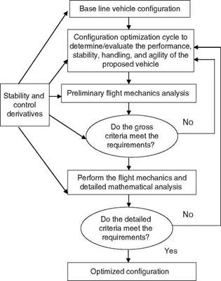
The lateral-directional derivatives are not influenced by longitudinal instability. However, the change in pitching moment due to change in AOSS (Cm ) plays an important role in the design cycle of unstable configuration. If it has a positive value, then it signifies the pitch up at moderate AOSS and can affect the Cm and Cm derivatives. Thus Cmft should be zero or negative up to ±15° of AOSS. In Figure 4.3 we see that there are certain criteria termed as gross and detailed criteria that are required to be met to obtain the final configuration of the vehicle. Gross criteria are based on the expert designer’s feel translated to some numerical values of the

derivatives that the configuration should possess. Once these criteria are satisfied, one proceeds to meet the detailed criteria. Some compound derivatives, as discussed in Section 4.3.3, based on basic derivatives are to be met in the gross criteria. The positive values of these compound derivatives are needed to ensure departure-free dynamic behavior of the aircraft up to maximum AOA. The detailed criteria need detailed mathematical analysis or simulation of dynamics to further ascertain their compliance. The derivatives play an indirect role in this process as they appear in TFs. These studies are also vital in the assessment of the stability and control characteristics of the aircraft, for which flight control laws need to be developed, especially for the inherently unstable configuration. The derivatives form important inputs to the control law development process and are also necessary to determine air loads on the vehicle. The study of aerodynamic derivatives is also important to assess the effect of changes in aircraft configurations (air brakes, slates, leading edge vortex control devices, etc.) and assessment of stores (like missiles, drop tanks, etc.). A further role of stability derivatives is in realizing the combat effectiveness of any fighter aircraft. The combat effectiveness is a function of

(a) Performance: sustained turn rate, specific excess power, and level speeds

(b) Agility: ability to change the state vector in the shortest possible time

(c) Maneuverability: roll performance, pullup, and roll pull out

(d) Operational boundaries: AOA-AOSS envelope restricted by recovery mar­gins, lateral-directional divergence angles, and pitch up

The primary dependence of these on stability derivatives is qualitatively presented in Table 4.10. From the foregoing discussions we see that aerodynamic derivatives, often called stability and control derivatives or in short, stability derivatives (and often only as derivatives), play a very crucial role in aircraft design cycles, perform­ance optimization, design and development of flight control laws, flight simulation, and many related analyses of aircraft (missiles) from flight mechanics point of view. We see that the information and knowledge from control and system theories play

TABLE 4.10

Relation of Derivatives to the Combat Effectiveness of a Typical Fighter Aircraft

Cm. , Cn. , CL

Singh, K. P. and Sreenivasan, M. N., Aerodynamic stability derivatives, Personal communications and notes, Hindustan Aeronautics Limited, Bangalore, 1990. With permission.

Besides the usual role these derivatives play.

an important role in the task of understanding and appreciating this design and development process apart from flight mechanics modeling and analysis.

In rotorcraft flight dynamics analysis, the same stability and control derivatives expressions as used in the aircraft analysis are used. Asymmetric cross-coupling derivatives are usually neglected in aircraft flight mechanics analysis; however, in rotorcraft analysis these are also used. For a rotorcraft, we have

1 dM

Iy dw

In this case, the controls are held at the trim values. Higher-order rotor DOFs are allowed to reach a new equilibrium. The conventional 6DOF derivative model is a poor approximation for rotorcrafts, since the dynamics of the rotor response are not well separated from airframe dynamic responses [7]. The use of the 6DOF quasi­static derivatives is found to give an impression of greater aircraft stability. This is so because the regressing flapping mode (of the rotor) is neglected. In flight, the rotor is continuously excited by control and turbulence inputs and the estimates from the flights might differ considerably from the analytical perturbation derivatives (e. g., WT derivatives). The main reason is that the linear rotor plus body models are not easily derived by analytical means. These models should be determined from more comprehensive nonlinear models. In addition, because of the lack of physical interpretation of the higher-order rotor plus body models, the use of quasi-static

TABLE 4.9 Most Important Missile Aerodynamic Derivatives With Respect to Component Velocities With Respect to Angular Velocities (Rates) With Respect to Control Surface Deflections Response Variables^ Forces/Moments, U V (Axial) (Side) w (Normal) p q r (Roll) (Pitch) (Yaw) Se (Elevator) 5a (Aileron) Sr (Rudder) X (axial) Y (side) Yv (—ve, 1/s) Cr, Yr (+ve, m/s) YSr (+ve, m/s2) CYSr Z (vertical/normal) Zw (-ve, 1/s) Zq (usually —ve, m/s) Zs, (-ve, m/s2) L (rolling) Lp (-ve) Cip (-ve, 1/s2) ClSp M (pitching) Mw (-ve, 1/m-s) СШа Mq (-ve, 1/s) Сша MS’ (—ve, 1/s2) cmst N (yawing) Nv (+ve, 1/m-s) C„ Nr (—ve, 1/s) c„r NSr (-ve, 1/ C„sr

derivatives persists in rotorcraft analysis [7]. In general forces/moments equations are given as follows, by representing the changes about the trim conditions as the linear functions of the rotorcraft’s states:

The first and second terms of Equation 4.45 are the perturbation accelerations due to the aerodynamic forces and moments. If the coupling between various axes is strong, then the rotorcraft has many more derivatives (say up to 36 force and moments derivatives and 24 control derivatives) than an aircraft. For example, if the coupling between roll and pitch axes is quite strong, then Lq and Mp will have significant values. Also, Xu is the drag damping derivative. The complete sets of EOMs of a rotorcraft were discussed in Chapter 3. The simplified equations and linear models that can be easily used for generating dynamic responses will be discussed in Chapter 5, where the meanings and utility of all these derivatives will become clear. It is emphasized again here that the meanings of these aerodynamic derivatives across aircraft, missile, and rotorcraft should remain the same, with some specific interpretations depending on the special interactions between various axes of the airplane. This will depend on the extra DOF entering the EOM, e. g., for a rotorcraft. As seen in Chapter 3, the longitudinal modes for helicopters with zero or low forward speeds are very different from the short period (SP) and phugoid modes (see also Chapter 5). This is because certain derivatives disappear for the hovering flight. The derivatives Xw, Mw, and Mw are negligible. Additionally, in the hovering condition, U0 = Np = Lr = Nv = Yp = Yr = 0, under certain conditions that will be discussed in Chapter 5. In Ref. [10] the numerical values of the 60 aerodynamic derivatives estimated from the flight test data using the parameter-estimation method for three helicopters (AH-64, BO 105, and SA-330/PUMA) are given. However, a good number of derivatives have very small or negligible values.

There are only two important derivatives in roll degree of freedom (DOF). Lp is the usual damping derivative in the roll, a change in the rolling moment due to a change in the roll rate. As usual it is negative in sign. It is often considered to have a constant value for a given Mach number and altitude. Due to positive roll rate, the change in the rolling moment is such that it will oppose this change in the roll rate and hence provide (increased) damping in the roll axis. It is usually defined as

In an aircraft the major contribution to this derivative is from wing; however, in the case of a missile this is not the case.

LSa is the aileron control surface effectiveness derivative. It is defined as

1.4.1.1 Yaw Derivatives

Effect of change in side speed v/AOSS:

(Yv, Np)

Yv is given as

It must be noted here that for a symmetrical missile the normal force coefficient for yaw has the same value as the Cz. This lateral force derivative should be calculated from the total force from the wings, body, and the control surfaces. It is presumed that the control surfaces are in a central position. Np is the force derivative Yv times the distance of center of pressure from the CG. As in the case of an aircraft this distance is known as the static margin. It is a measure of the static stability of the missile. In the usual manner the derivative is defined as

It will change sign for an unstable missile configuration.

Effect of change in yaw rate r:

(Yr, Nr)

Yr is a difficult derivative to calculate and measure and hence it is usually neglected. Nr is given as

n = rUSb2 c

1У r y~-nr

with the usual definitions as in the previous case. It is a damping derivative in yaw. It has a small value.

Effect of change in rudder control surface deflection:

(YSr, NSr)

Ys is the side force derivative due to deflection of the rudder control surface. Nd is the yawing moment derivative due to deflection of the rudder control surface. It has the opposite sign for a missile with canard control surface. It is given as Yd times the distance of the center of pressure of the rudder from the CG. The formats of these derivatives are usually similar to the ones for aircraft.

Table 4.9 gives the most important missile aerodynamic derivatives. It can be observed that a missile has very few derivatives that are essential to describe its dynamics, especially from the control point of view. It will be a good idea and exercise to establish the equivalence between the formulations of Tables 4.5 and 4.8. We further illustrate this as follows since acceleration = force/mass:

day dFy @8 =

d(qSCy) pU2SdCy PU 2SCyb Y m@8 2m@8 2m 8

The normal force is given by Z = 1/2 pU[1] [2]SCz. Here, the area S is the maximum body cross-section reference area. Cz is the normal force coefficient and is a function of AOA (called incidence in pitch) for a given altitude and Mach number.

Za is defined as

— pU2SCZ, 2m Za

or

Zw = 2m pUSCza

The actual values of the normal force coefficient depend on the shape of the missile and the reference area S. The normal force coefficient for a missile is expressed in the literature as [5]

CN = CN0 + CNaa + CN, 2V + CNa( 2V ) + (4.38)

Here, V is the resultant velocity or the cruising speed of the missile. The parameter c is the total body length of the missile. In the case of the missile N denotes the normal force unlike for aircraft where Z denotes the vertical force. We use Z for the normal force uniformly. The meanings of the derivatives do not change.

Mw and Mq have the same significance as in the case of aircraft aerodynamics. Md will have an opposite sign for a missile with canard control surface (in the front). Mw will also change sign in case of an unstable missile configuration. Zd is related to Md in the usual manner and both are elevator control surface effectiveness derivatives. The derivative Zq is of no practical significance and hence neglected in missile aerodynamics.

1.4.1 Lateral-Directional Derivatives

TABLE 4.8

Missile Derivatives in a Linear Model

Changes in Variables

Pitch angular acceleration

Roll angular acceleration Yaw angular acceleration Normal (pitch) acceleration, az Axial acceleration, ax Yaw acceleration, ay

by mass m and the moment derivatives are divided by respective moment of inertia. A complete linear derivative model of a missile could have 30 derivatives [9] as shown in Table 4.8.

Interestingly these derivatives of Table 4.8 are called acceleration derivatives. The reason will be clear from the following development:

8U _ pU2Sc 8a 2Iy ‘

We know from Equation 4.7 that

Hence, 8a = Ma and we see that the corresponding derivative is also called pitch angular acceleration derivative. Similarly, all other derivatives of Table 4.8 can be shown equivalent in their formats by their definitions to aircraft derivatives. Some additional derivatives seem to have been defined in the case of a missile as can be seen from the Table 4.8, as compared to aircraft.

Two important compound derivatives are defined as [8]

(a) Cnbdynamic Cn$ cos a (1zz = 1xx)Clp sin a (4-33)

This compound derivative contains Cn and Ci static stability derivatives. This derivative will be the same as the weathercock stability if the AOA is zero or negligibly very small. For reasonably small AOA we have

Cng dynamic Cng — (1zz/1xx)Clba

TABLE 4.6

Typical Values of Some L-D Derivatives for a Small Trainer Aircraft

TABLE 4.7

Typical Values of the Compound Derivatives for a Supersonic Fighter Aircraft

Flight condition: Mach — 0.55, altitude — 6 km, and trim AOA — 6°.

For Dutch-roll static stability should be positive. At high AOA it

might become negative as can be seen from the above expression, thereby affecting the stability adversely.

(b) Lateral control divergence parameter (LCDP)

LCDp — Cnp (CnSa =CiSa )Cib

This parameter should be positive to avoid reverse responses due to adverse aileron yaw.

The positive values of the compound derivatives are necessary up to a maximum AOA for ensuring departure-free behavior of the aircraft. For nonzero AOA both the derivatives should be studied and the stability should be guaranteed. Typical numer­ical values of these compound derivatives are given in Table 4.7.

DADs are directly related to the forces and moments as well as to the aircraft response variables. DADs are useful as they directly appear in the simplified EOM/differential equations, which describe the vehicle dynamic responses as will be seen in Chapter 5. That is to say that DADs appear in TF models that can be used to describe the dynamic responses/Bode diagrams for the aircraft in a particular axis in an approximate way. NDADs are directly related to the aerodynamic coefficients and nondimensional velocities (Tables 4.3 and 4.4). The merits of nondimensional forms are (1) easy correlation between the results from different test methods like WT, flight tests, theoretical predictions (CFD, DATCOM), (2) correlation between the results from different flight test conditions, and (3) possible comparison/correla – tion of the results of different configurations of the same aircraft or different aircraft of similar kind (or even other kinds). DADs and NDADs defined and studied here can be very conveniently used in aerodynamic models of atmospheric flight vehicles.