Category FLIGHT MECHANICS MODELING and ANALYSIS

Lateral-directional derivatives are defined as the sensitivities of the side force, the rolling moment, and the yawing moment with respect to small changes in side speed, roll rate, yaw rate, and aileron – and rudder-control surface deflections. These deriva­tives are, in general, difficult to estimate with a good degree of confidence.

Effect of change in side speed v/AOSS:

(Yv, Lb, Nb)

Yv is the change in the side force due to a small change in the side velocity v. The side force Y is given by

pu2sc 2 Cy

and hence pU2S dCy

2 ~dv

Using v = bU, we obtain

This derivative is difficult to estimate. It is usually negative, since sideslipping causes the side force that opposes the sideward motion.

Lb is the change in the rolling moment due to a change in sideslip. We have

Ci is the effective dihedral and it is negative for the positive dihedral. It is essential for lateral stability and control and hence considered as a preliminary design parameter.

Nb is the change in the yawing moment N due to a change in the side velocity. It is mainly caused by the side force on the vertical tail. Following the previous development for Lv, we obtain

pUSbc 2Іг Cnb pU2Sbc 2I7 Cnb

The vertical tail and related lever arm contribute to Cn. This contribution is positive and signifies the fact that due to positive sideslip this force creates a positive yawing moment, which in turn tries to reduce the sideslip thereby maintaining the static stability.

Effect of change in roll rate p:

(Yp, Lp, Np)

These derivatives arise due to the change in rolling angular velocity, roll rate p. The roll rate creates a linear velocity of the vertical, horizontal, and wing surfaces, causing a local change in the AOA of these surfaces and the lift distribution, which in turn causes the moment about the CG.

Yp is the change in side force due to a change in the roll rate. We have

PUSbr 4m CYp

This derivative is not significant and is often neglected.

Lp is the change in the rolling moment due to a change in the roll rate p. It is known as a roll-damping derivative. The induced rolling moment is such that it opposes the rolling moment thereby providing dynamic stability to the aircraft. We have

pUSb2 dr 4Ix @( pb/2U)

(1/Ix)dL/dp

(4.27)

x

Np is a change in the yawing moment due to a change in roll rate. It is given as

with usual definitions as in the previous case.

Effect of change in yaw rate r:

(Yr, Lr, Nr)

The yawing angular velocity, yaw rate, causes these derivatives. The yaw rate causes the change in the side force that acts on the vertical tail surface.

Yr is the change in side force due to a change in the yaw rate. We have

(1 /m)dY/dr

pUSb 4m 4r

Lr is the change in the rolling moment due to a change in the yaw rate r. We have

Nr is a change in the yawing moment due to a change in yaw rate. It is given as

with usual definitions as in the previous case.

Effect of change in aileron and rudder control surface deflection:

(YSa, LSa, NSa, YSr, LSr, NSr)

Ls and N8 are the primary control derivatives or control power. If the absolute magnitude of these derivatives is higher, then for a given deflection, more rolling and yawing moments are generated. This is regarded as higher control sensitivity for a given moment of inertia.

YSa = (1/m)d Y /88 a =

Similarly,

Ydr = (1/m)8Y/88r = ^ CySr (4.32)

N8 and L8 are cross-derivatives and will be useful if there is rudder-aileron inter­connect for certain high-performance fighter aircraft or rotorcrafts.

Some important derivatives are explained next.

(a) Cn represents the directional static stability. If Cn > 0, then aircraft possesses static directional stability. Such an aircraft will always point into the relative wind direction and hence the directional stability is also called the weathercock stability, synonymous with the concept of the weathercock at airports, etc. At high angles of attack (HAOA) Cn will be affected significantly because the fin will get submerged in the wing – body wake. This derivative is of significant importance in dynamic lateral stability and control. It governs the natural frequency of the Dutch-roll oscillatory mode of the aircraft. It also contributes to the spiral stability of the aircraft.

(b) Ci is the rolling moment derivative (due to a small change in AOSS). It provides the dihedral stability for C < 0. The dihedral instability will contribute to the spiral divergence. A stable dihedral will tend to decrease the AOSS by rolling into the direction of yaw. Both C and Cn affect the aircraft Dutch-roll mode and spiral mode as will be discussed in Chapter 5.

(c) Ci is the damping-in-roll derivative and determines roll subsidence. The change in rolling velocity causes the change in rolling moment. The +ve roll rate induces a restoring/opposing moment and hence the derivative has generally —ve magnitude. It can also be considered as a design criterion, since it directly affects the design of ailerons.

(d) Cn is a cross-derivative that influences the frequency of Dutch-roll mode.

(e) Cn is the damping-in yaw parameter that contributes to damping of the roll-roll mode in a major way.

(f) Ci affects the aircraft spiral mode.

(g) Ci and Cn are important derivatives that represent the aileron control effectiveness and the adverse yaw derivative, respectively. Cn is an important lateral-directional control derivative.

(h) Cys, Chr, and C,

Cn is an important lateral-directional control derivative representing rudder effectiveness. Numerical values of certain lateral-directional derivatives are given in Table 4.6.

These derivatives are related to the sensitivities of the forces in axial and vertical (normal) directions and the pitching moment with respect to changes in forward speed, normal speed, pitch rate, and elevator/elevon control surface deflections.

Effect of forward/ axial speed u:

(Xu, Zu, Mu)

When there is an increase in the axial velocity the drag and lift forces generally increase. Also, the pitching moment changes. Let us consider the effect of change in forward speed of the aircraft on the lift, drag, and pitching moment.

Xu is the change in forward force (often known as the axial force) due to a change in the forward speed (also known as the axial speed). It is called the speed-damping derivative. By definition, following Equation 4.7 (for force derivatives mass m is

control surface deflection.

1 @M _ pSU2c dCm

Ty me – 2iy ~we

pSU2cC

2Iy mge

Cmg derivative can be considered as a primary design parameter and it specifies longitudinal axis control power. Important and routinely used longitudinal DADs and NDADs (stability and control derivatives) are given in Table 4.3 in a compre­hensive format. Some important longitudinal derivatives are explained next.

(a) CL is defined as a change in lift coefficient for a unit change in AOA. The lift force can be easily given by

L = CLqS

CL represents the lift-curve slope with respect to AOA. This is a very important derivative because it almost directly determines the contribution to the lift force. It also signifies the fact that as AOA increases, the lift force increases proportionally in the linear region up to a certain AOA. Beyond this AOA the lift would remain somewhat constant and would even decrease further. This condition is called ‘‘wing stall’’ (Appendix A). This means that the aircraft loses some lift after it stalls.

(b) Cm is the basic static stability derivative and is also referred to as the pitch stiffness parameter [2]. A negative value of Cm indicates that the aircraft is statically stable, i. e., if the AOA increases then the pitching moment becomes more negative, thereby decreasing the AOA and hence restoring the stability. Cm derivative is proportional to the distance between the aerodynamic center (better referred to and used as neutral point, NP) of the aircraft and the CG. This distance is related to the static margin as

Static margin = (NP distance — CG)/MAC

The distances (of NP and CG) are from some reference point in the front of the aircraft on the x-axis. If the static margin is positive, then the aircraft is said to have static stability. This means that the NP distance is larger than the CG distance from the reference point. If the CG is continuously moved (by some means) rearwards, then at one point the aircraft will become neutrally stable (neutrally unstable!). This point is called the NP of the aircraft or this CG position/location is called the NP. The NP must always be behind the CG location for guaranteed static stability. A slightly more rearward movement of the CG will render the aircraft statically unstable. If the aircraft is dynamically stable then it must have been statically stable. For dynamic stability the static stability is a must, but the converse is not true, meaning that if the aircraft is statically stable it could be dynamically unstable. This derivative is of primary importance to the longitudinal stability of atmospheric vehicles. If the aircraft is inherently statically unstable (by design or for gaining certain benefits in case of a relaxed static stability aircraft like FBW and many modern-day high – performance fighter aircraft), then artificial stabilization is required for the aircraft to fly. The level of instability is dictated by (1) available state-of – the-art technology (computers, actuators, sensors, and control law design tools), (2) possible reduction in the size of the aircraft and subsequent decrease in weight, (3) increase in weight due to additional hardware (redundancy, computer, etc.), (4) obtainable performance, (5) maneuver­ability, and (6) agility. This is the subject of design and development of flight control laws.

(c) Cm signifies a change in pitching moment coefficient due to a small change in pitch rate q. Being (angular) a rate-related derivative it implies, from the control theory point of view, that it must have something to do with damping-in pitch. As such it contributes to the damping-in pitch. Usually more negative values of Cm signify increased damping. The sign is gener­ally negative for both stable and unstable configurations. Since the statically unstable configurations will have stability augmentation control laws, the lower values of this derivative (less —ve values) are acceptable. The aircraft flight-control system (AFCS) also provides some artificial damping. This derivative often has higher prediction uncertainty levels (scatter in esti­mates); however, this is not a problem since AFCS generally tolerates these uncertainties.

(d) Longitudinal control effectiveness derivative Cm is the elevator control effectiveness. In conventional sense, more negative value means more control effectiveness. It also helps determine the sizing of the control surface. More elevator (elevons for FBW delta-wing aircraft configuration) control power means more effective control in generating the control moment for the aircraft. This also applies to horizontal tails, canard, or a combination of these surface movements. The knowledge of the available elevator/elevon power at all the flight conditions (Chapter 7) in the flight envelope is extremely important. The unstable configurations demand higher control power than the stable ones. Numerical values of certain longitudinal derivatives are given in Table 4.4.

Important lateral-directional aerodynamic derivatives are collected in Table 4.5 in a comprehensive and compact manner, along with brief explanations and indication of influence of certain derivatives on aircraft modes.

Essentially these derivatives are sensitivities to changes in flight variables. A change in AOA results in a change in the pitching moment coefficient and an appropriate change in the pitching moment M (see Equation 4.2). How this change in turn alters the aircraft responses is the subject of the EOM (Chapters 3 and 5). There could be cross-coupling terms, i. e., a change in the aerodynamic coefficient of one axis due to a change in the variable of the other axis. Several possibilities exist. The analysis is limited to straightforward effects. The force and moment coefficients of Equations

4.1 and 4.2 are expressed in terms of the aerodynamic derivatives as seen in Equation 4.6. These are often called stability and control derivatives. This is because they directly or implicitly govern the stability and control behavior of the vehicle. They are called derivatives as they specify the variation of aerodynamic forces and moments with respect to a small change in the perturbed variable. A particular derivative could vary with velocity or Mach number, altitude, and AOA. And in turn the coefficients that depend on these derivatives also vary with these and several other variables. However, the variation of these coefficients soon gets translated to variations with time because of the composition of the coefficients in terms of motion variables, which vary with time.

Table 4.1 gives the matrix of relationships in terms of the sensitivities between the forces/moments and the response variables u, v, w, p, q, r, and control surface deflections in terms of the aerodynamic derivatives. Table 4.2 depicts the major functional (effect) relationships between forces/moments and the aircraft response variables and classifies them broadly as mentioned in the table. In other words, we have the following classification: (1) speed derivatives, (2) static derivatives, (3) dynamic derivatives, and (4) control derivatives. The static derivatives are mainly with respect to AOA and AOSS. They govern the static stability

09 09

TABLE 4.1 Relationship Matrix for Forces/Moments and the Independent Response Variables With Respect to With Respect to Angular With Respect to Control Component Velocities Velocities (Rates) Surface Deflections Response Variables^ Se (Eleven/ Forces/Moments J. и (Axial) v (Side) w (Normal) p (Roll) q (Pitch) r (Yaw) Elevator) Sa (Aileron) 8, (Rudder) X (axial) xu Aw X» Xs, Cd, Cd<x Cds, Y (side) Yv YP Yr Ysa Ys, Суs Cyp Су, Cysa Crs, Z (vertical/normal) zu Zw zq Ze, Си cLa Cl, Cls, L (rolling) LP Lp L, LSa Ls,. Cl„ Qp Q, Cm, Cm, M (pitching) Mu Mw Mq Ms, Сш, c Аша Сш, Cm8e N (yawing) Np Np N, NK Ns, Cn„ c ‘-■np c ^nr CnSa Cn8,

(Appendices A and C) of the vehicle. Dynamic derivatives are with respect to the rotational motion of the vehicle and mainly specify the damping (of certain modes of the vehicle) in the respective axis. The speed derivatives are with respect to linear velocities of the vehicle. The control derivatives specify the control effect­iveness of the control surface movements in changing the forces and moments acting on the vehicle.

We see from Table 4.2 that the static and the dynamic derivatives, as they are termed, imply something definitely more in terms of the behavior of the aircraft from control theory point of view (Appendix C). What is important to know is that these names themselves relate to certain stability and damping properties of the aircraft, which is considered as a dynamic system. This aspect is further explored in Chapter 5.

The derivative effects are considered in isolation assuming that the perturbations occur in isolation. The aerodynamic derivatives are evaluated at steady-state equi­librium condition with a small perturbation around it. Hence, these derivatives are called quasi-static aerodynamic derivatives. Interestingly enough, these derivatives are used in dynamically varying conditions also, mainly for small amplitude man­euver analysis, thereby assuring the linear domain operations and analysis. For large amplitude maneuvers where AOA are high, the unsteady and nonlinear effects need to be incorporated into the analysis for which additional aerodynamic derivatives must be included. For definition of dimensional aerodynamic derivatives (DADs) and nondimensional aerodynamic derivatives (NDADs) we closely follow Ref. [2] because the definitions and procedures therein are consistent and straightforward. The present study is also enhanced by the research presented in Ref. [3,5-9]. Although there might be some differences in the formulae of certain derivatives between various sources [2,3,5-9], the presentation in this book is more uniform and highly standardized as in Ref. [2]. DADs are defined as

The derivatives specify the change in pitching moment/vertical force due to a small change in vertical speed (w) of the aircraft. Next, we have NDADs defined as

since Cm = M/(qSc) and a = w/U (for small alpha), we get

dM 1

d(w/U) qSc U dM qSc dw

Щ

qSC

Finally, we get

Mw = qSc/(IyU)Cma

= pUS-c/(2Iy )Cma (4.9)

A similar procedure can be applied to all the dimensional derivatives to obtain the equivalent nondimensional derivatives. The decoupling between longitudinal and lateral-directional derivatives is presumed. We also assume that during a small perturbation maneuver, the Mach number, Reynolds number, dynamic pressure, velocity, and engine parameters do not change much, so their effects can be neglected.

The important longitudinal aerodynamic derivatives are collected in Table 4.3 in a comprehensive and compact manner along with brief explanations and an indica­tion of the influence of certain derivatives on aircraft modes.

The aerodynamic coefficients would, in general, be a function of not only the flow angles but also of Mach number, angular rates, control surface deflections, and changes in thrust force due to the movement of the throttle lever arm. For example, Cm from Equation 4.2 can be expressed in terms of these independent response variables in a straightforward manner as

Cm = function of (a, q, 8e, M, FT)

= Cm0 + Cmaa + Cmq F Cmde de + CmMM + CmFjFT (4-6)

Here, the pitching moment aerodynamic coefficient is considered a function of several independent variables: AOA, pitch rate q, elevator control surface deflec­tion, Mach number, and thrust. The effect on the pitching moment, due to small changes in these response variables, is captured in terms that are called aerodynamic derivatives (e. g., Cm ). These terms can be considered proportionality constants. However, these constants vary with certain variables. The quantity is the non­dimensional angular rate (velocity) as can be seen from (rad/s) (m/2) (s/m) => rad. The small perturbation theory when applied to the simplification of the EOM leads to the fact that the aerodynamic forces and moments depend on some constants that are called stability derivatives. The parametric terms of Equation 4.6 are called aerodynamic derivatives, and often stability and control derivatives, as many of these derivatives govern the stability and control of the aircraft (dynamics), as will be shown later. For example, Cm signifies -—у when other variables are set to zero.

It is apparent from Section 3.2 that if we specify certain geometric parameters of the aircraft like reference surface area of the wings S, the mean aerodynamic chord C, the wing-span b, and the dynamic pressure q (Appendix A), then we have the following straightforward aerodynamic force and moment equations:

Force = pressure x area

Fx = CxqS

Fy = CyqS (4.1)

Fz = CzqS

These equations are in terms of the component forces in x, y, and z directions. Moment = force x lever arms (respective ones):

L = CiqSb

M = CmqSc (4.2)

N = CnqSb

These expressions are in terms of the component moments: rolling moment L about the x-axis, pitching moments M about the y-axis, and the yawing moment N about the z-axis (see Appendix A for geometry of b and qc used as appropriate lever arms for defining the moments). Here, Cx, Cy, Cz, Cl, Cm, and Cn are the nondimensional body-axis force and moment coefficients, and are called aerodynamic coefficients. They are the proportionality constants (that actually vary with certain variables) in Equations 4.1 and 4.2. The dynamic pressure is q = 1/2pV2 in terms of air density p
at an altitude and air speed V. Actually V is the total velocity of the air mass striking the vehicle at a certain (total) angle, and both the velocity V and the total angle can be resolved as shown in Figure 4.2 in terms of component velocities: u, v, and w and AOA and AOSS (Appendix A).

From the geometry of the flow velocity (Figure 4.2) the following expressions of the flow angles and component velocities emerge very naturally:

і w

a = tan

u

v

b = sin-1 V

as AOA (in vertical x—z plane) and AOSS (in horizontal x—y plane), respectively. By trigonometric transformation we get equivalent expressions as

u = V cos a cos b

v = V sin b (4.4)

w = V sin a cos b

The total velocity V of the airplane is expressed as

V = J u2 + v2 + w2 (4.5)

in terms of its components u, v, and w. From the basic definition of pressure and force, we have come to some more details of the interplay of flow angles, compon­ents of the total velocity, and aerodynamic coefficients. We must emphasize here that discussing the three components of the total velocity in the three directions is equivalent to considering that the airplane experiences motion along these three axes. Thus, we have put the airplane in real motion in air. What actually keeps the airplane lifted in the air is the lift force (Appendix A).

Now, if the values of the aerodynamic coefficients are known, then the forces and moments acting on the aircraft can be determined easily, since V and the geometrical parameters like area and lever arms are known. Alternatively, if we know the forces by some measurements on the aircraft, then the aerodynamic coefficients can be determined. Actually, the latter is true of the WT experiments conducted on a scaled model of the actual aircraft. In a WT, the model is mounted and compressed air is released, thereby putting the model in the flow field. The experiments are conducted at various AOA and AOSS settings, and forces and moments are measured/calculated from equivalent measurements. Since the flow velocity and the dynamic pressure are known, simple computations would lead to the determination of the aerodynamic coefficients. One can see that these coefficients can be obtained as a function of flow angles, Mach number, etc. Similar analysis can be done using CFD and other analytical methods (Appendix A). To determine the aerodynamic coefficients from experimental/flight data we need to know V and measure the force, i. e., force = mass x acceleration. Since mass is known, acceleration can be obtained as qSCx. Therefore, if the acceleration of an airplane in motion is measured, the aerodynamic coefficient Cx can be obtained. Since the coefficients depend on aerodynamic derivatives and dynamic variables, and by measuring these responses, these derivatives can also be worked out. This calls for establishing the formal relationship between these dynamic responses and the aerodynamic derivatives, thus leading to aerodynamic modeling.

The pilot will maneuver an aircraft using the pitch stick, roll stick, and rudder pedals besides using the throttle lever arm. The movements of these devices forward, backward, or sideways are transmitted via the control actuators to the moving/hinged surfaces of the aircraft. These surfaces are extensions of the main surfaces, like wing, rudder fin, etc., and are called control surfaces. The movements of the control surfaces interact with the flow field while the aircraft is in motion and alter the force and moment balance (equations), thereby imparting the ‘‘changed’’ motion to the aircraft until the new balance is achieved. During this changing motion (which can be called perturbation), the aircraft attains new altitude, acquires new orientation, etc., depending on the energy exchanges and balance between kinetic, potential, and propulsive (thermal) energies. At microscopic level (or scale) this behavior can be studied by exploring the effect of the aerodynamic param­eters discussed in the following section. At the macroscopic level (or scale) the behavior can be studied using the simplified EOM and resultant transfer function (TF) analysis. Hence, we gradually get closer to flight motion and hence flight mechanics.

4.1 INTRODUCTION

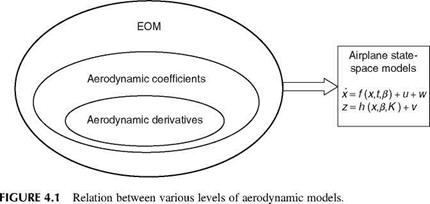
Apart from the equations of motion (EOM) discussed in Chapter 3, the quantification and analysis of aerodynamic models is most important for flight mechanics analysis. The forces and moments that act on an aircraft can be described in terms of aerodynamic derivatives. The stability and control analysis is an integral part of aircraft design cycles, design evaluations, and design of control systems. In this analysis, the aerodynamic derivatives, often also known as stability and control derivatives, form the basic inputs [1-3]. For conventional stable aircraft configur­ations these derivatives directly ensure the required levels of stability and control­lability. For unstable aircraft configurations these derivatives form the essential input parameters for the design of control laws, which in turn ensure the desired stability and controllability characteristics of the aircraft. Stability derivatives also play an important role in the selection process of aircraft configuration, as will be seen in Section 4.4 [4]. This aerodynamic model then becomes an integral part of the EOM that in totality represents the aerodynamics as well as the dynamic behavior of the vehicle. The accuracy of the results of any flight mechanics analysis depends on the degree of completeness and approximation of the aerodynamic models used for such analysis. Due to the assumption of linearity often made, the validity of these models (the EOM and aerodynamic models) is limited to a small range of operating conditions. These operating conditions are generally in terms of the angle of attack (AOA) and Mach number. Often the excursion in the angle of sideslip (AOSS) is assumed to be small. In general, aerodynamic derivatives are applicable to small perturbation motion about a particular equilibrium and this leads to quasi-static aerodynamic derivatives. Large amplitude motions and maneuvers require sophisti­cated and complex aerodynamic modeling. In this chapter we deal with aerodynamic modeling, which basically consists of aerodynamic coefficients that in turn expand to (or encompass) aerodynamic derivatives. Certain stability and control aspects (of aircraft) are captured in certain aerodynamic derivatives. Primary knowledge of aerodynamic coefficients, especially of aerodynamic derivatives, can be obtained from some analytical means like DATCOM, CFD, and wind-tunnel (WT) experi­ments (Appendix A). When flight tests are conducted on an airplane and if they instrumented properly with sensors, one can measure the dynamic responses (p, q, r, AOA, AOSS, Euler angles, and linear accelerations) of the aircraft when certain maneuvers (Chapter 7) are performed. These responses/data can be processed using parameter-estimation methods to obtain the aerodynamic coefficients/derivatives

(ACDs), as will be discussed in Chapter 9. The interplay of aerodynamic coeffi­cients, derivatives, and EOM at the top level is shown in Figure 4.1.

The 6DOF model in Equations 3.44, 3.46, 3.47, and 3.50 involving the rigid body states is generally adequate to predict rotorcraft dynamics in low – and mid-frequency range. In the conventional rigid body model, the main rotor dynamics are omitted and the rotor influence is absorbed by the rigid body derivatives. A better prediction at higher frequencies, however, necessitates the inclusion of rotor dynamics in the estimation model. One approach to include rotor effects in a 6DOF model is introdu­cing equivalent time delays in control inputs [11,12]. These delays can be determined by correlating model response with flight data. This is, however, an inappropriate alternative to modeling the rotor dynamics, which are highly complex in nature. Model inversion is required for the feed forward controller in the design of a model following control systems and the time delays become time lead on inversion, which means that the future values of the state variables are needed in advance. This is unrealistic for an online real time process like in-flight simulation. It clearly underlines the need to develop extended models with an explicit representation of rotor dynamic effects. Therefore, the 6DOF rigid body model is generally extended with additional degrees of freedom representing the longitudinal and lateral rotor flapping.

The basic approach to extend the 6DOF rigid body model is shown in Figure 3.16. The model structure now includes two additional degrees of freedom

representing the longitudinal and lateral flapping [10,11]. The state-space matrix in Figure 3.16 defines the submatrices pertaining to rigid body, rotor, and the cross-coupling matrices for body-to-rotor and rotor-to-body. In a simplified rotor model, the longitudinal and lateral flapping angles can be expressed primarily as a function of body angular rates and control inputs. In Ref. [12], Kaletka et al. formulated an 8DOF extended model by redefining the roll and pitch acceler­ations for rotor/body motion and using them as state variables. Tischler provided a hybrid body/flapping model, which coupled the simplified fuselage equations at low frequencies to the simplified rotor equations at high frequencies with equiva­lent spring terms [13]. The following first-order coupled differential equations for longitudinal flapping a1s and lateral flapping b1s can be appended to the 6DOF model:

a 1s = A; b 1s = B (3.51)

Here, A and B are the longitudinal and lateral flapping-specific moments.

EPILOGUE

An extensive treatment of EOMs is found in one of the earliest books [1]. Extensive helicopter research work on aeromechanics is reported in Ref. [14]. It takes a systems approach and deals with three major aspects of helicopter research, which are also equally applicable and suitable to fixed wing aircraft research and development: (1) reality and conceptual model linking through wind tunnel simulation—this is analysis route (Appendix A, Chapter 4), (2) linking of conceptual model (Chapters 3 and 5) and computerized model via model verification—this is the programming route, and (3) linking of computerized model and back to the reality via system identification/model validation procedure—this is the computer simulation route (Chapters 6 and 9).

Models of different order may be used depending on what is known about the measurements available, the frequency range of interest, and the degree of coupling between the longitudinal and lateral-directional motions. Generally, a 6DOF model is the minimum required for a highly coupled rotorcraft. The 6DOF rigid body model for rotorcraft consists of the usual EOM derived from Newton’s law.

Equations for linear accelerations

U = X — g sin U — qw + rv

v = ~ + g cos U sin f — ги + pw (3.44)

W = Z + g cos U cos f — pv + qu

Equation 3.45 can be further simplified by assuming the product of angular rates to be small and neglecting the corresponding terms in the moment equations. Equation 3.45 in that case reduces to the form

P = L

q = M (3.50)

r = N

The rigid body states described in Equations 3.44, 3.46, 3.47, and 3.50 are used to characterize rotorcraft dynamics. Since the forces and moments are presented as specific quantities in the equations, mass and moment of inertia no longer explicitly appear in the mathematical model.

The momentum theory discussed here provides an estimate of induced power requirements for the rotor, but is not sufficient for designing the rotor blades. The origin of blade-element theory can be traced back to the work on marine propellers by Froude. Subsequently, Drzewiecki took up this study assuming the blade sections to act independently and considering two velocity components VR due to rotation and V due to the axial velocity of the rotor. His results indicated correct behavior but were quantitatively erroneous, which was primarily due to neglecting the induced velocity at the rotor disk [10].

Several attempts were made later on to account for the induced velocity from momentum theory into the blade-element theory. It was only after Prandtl developed the lifting line theory that the influence of the wake velocity at the rotor disk was incorporated. Thus, it was through the wake vortex theory rather than the momentum theory that the induced velocity at the blade section was finally incorporated into the blade-element theory. The blade sees the air coming to it due to rotor rotation, as well as due to downward-induced velocity. Today, the blade-element theory is the foundation for all analyses of helicopter dynamics and aerodynamics. Reference [8] describes in detail the blade-element theory for a rotor in vertical flight.

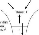
The momentum theory follows the basic laws of conservation of mass, momentum, and energy [9,10]. The action of the air on the rotor blades produces a reaction of the rotor on the air, which manifests in the form of thrust at the rotor disk. It is assumed that the rotor disk is composed of infinite number of blades, i. e., the rotor is considered to be an ‘‘actuator’’ disk. It is also assumed that the air is incompressible and frictionless and no rotational energy is imparted to the flow outside the slip­stream. Velocity in the slipstream increases from zero at upstream infinity to v at the rotor disk and to w at downstream infinity (Figure 3.15). For air with density p and A the disk area, the law of conservation of mass gives

rn = pAv

P<

FIGURE 3.15 Flow across the actuator.

If T is the thrust at the rotor disk, it will be equal to the rate of change of momentum, i. e.,

T = m (w — 0)

= pAvw (3.37)

From the law of conservation of energy, we have

T v = 1 mw2 (3.38)

Substituting for T from the momentum conservation equation, we have

pAvwv = 2 pAvw2

or

v = 2 w (3.39)

Thus, the velocity at downstream infinity is twice the velocity at the rotor disk. From the momentum conservation equation, the relation between v and thrust T now becomes

T = pAv2v

or

The term “T/A” is also known as disk loading. The induced power for the rotor can be written as

T

P = T v = TJ——–

V 2pA

In nondimensional form, thrust and power coefficients are given by

Here, V is the angular velocity and R is the radius of the rotor.

The inflow ratio l is given by

The hovering efficiency of the rotor is defined by figure of merit M, defined as

minumum power required to hover
actual power required to hover

The ideal value of M is equal to 1. However, for most rotors, the value lies between 0.75 and 0.8.