Category FLIGHT MECHANICS MODELING and ANALYSIS

As mentioned above, rotorcraft applications require at least a 6DOF model to represent the rigid body motion. Such models are generally adequate to describe helicopter dynamics associated with low frequency (such as phugoid). However, the prediction of flight dynamic behavior from such models in the high-frequency range is poor. This is due to the absence of the rotor degrees of freedom in the model, which effect the helicopter motion. Some improvements can be obtained by approxi­mating rotor dynamics via equivalent time delay effects [7]. However, this approach cannot adequately represent the rotor influences [8]. The other alternative is to augment the 6DOF models with additional degrees of freedom that explicitly model the rotor dynamic effects, e. g., longitudinal and lateral flapping and coning. Figure 3.16 shows the submatrices that define body, rotor, and body-rotor coupling. An extended model of 8DOF can be obtained from Equation 5.38 by including longitudinal and lateral flapping in the state and observation equations [9].

xT = (u, v, w, p, q, r, f, U, ф, h, as, bs)

y (axm, aym, azm, pm, qm, rm, fm, Um, um, vm, wm, pm, qm, rm, Фт, hm, a1s, b1s)

UT = (dlon, dlab dcob dped) (5-40)

In comparison to the 6DOF rigid body model, this extended model structure can provide an in-depth insight into helicopter dynamics. However, the augmented model will have larger number of unknowns to be estimated which can lead to serious convergence problems and make identification difficult. The rotorcraft mathe­matical model should be such that it gives a realistic representation of the helicopter behavior and at the same time is simple and mathematically tractable. To this end, it is essential to determine the lowest-order model that would best fit the flight test data. Linear models of different order, which may include body as well as rotor degrees of freedom, can be tried out in identification. Any one of the following model structures, consistent with the frequency range of interest, can be selected for characterizing rotorcraft dynamics [10,11]:

• Body longitudinal dynamics alone—fourth-order model (3DOF)

• Body lateral dynamics alone—fourth-order model (3DOF)

• Body coupled dynamics—eighth-order model (6DOF)

• Body dynamics with first-order flapping dynamics—longitudinal and lateral tip path plane tilts—11th-order model (9DOF)

• Body dynamics with rotor flapping dynamics—15th-order model (10DOF)

• Body dynamics with rotor flapping and lead-lag dynamics—21st-order model (13DOF)

• Body dynamics with rotor flapping and lead-lag dynamics and with inflow dynamics—24th-order model (16DOF)

A general state-space form of a model to describe rotorcraft dynamics may be written as

x = f [x(t),u(t),Q] + Fw(t)

y(k) = g[x(k),u(k),Q] + Gv(k) (5.36)

x(0) = X0

The above is the mixed form of continuous-discrete state and observation equations, where x is the state vector, y is the measurement vector, u is the control input vector, Q is the vector of unknown stability and control derivatives, F is the state noise matrix, and G is the measurement noise matrix.

The linear form of the above state-space model can be expressed as

x = Ax(t) + Bu(t) + Fw(t)

y(k) = Cx(k) + Du(k) + Gv(k) (5.37)

x(0) = x0

where A and B are the matrices containing the stability and control derivatives and C and D are the matrices that relate the measured quantities to the rotorcraft states and control variables.

The 6DOF EOMs for modeling rotorcraft dynamics were discussed in Equations 3.44 through 3.47. From these equations and from the state-space model described in Equation 5.36, it is evident that the state, measurement, and control vector will include the following motion variables:

x = [u, v, w, p, q, r, f, U, h]

y [um, vm, wm, pm, qm, rm, fm, Um, hm, axm, aym, azm, pm, qm, rm] (5.38)

u [dlon, dlat, dcol, dped]

The structure of the Equations 3.44 through 3.47, is nonlinear due to the presence of gravity and rotational terms in Equation 3.44 and due to the presence of the product of angular rates in the moment equations given by Equation 3.45.

Assuming small variations in u, v, w, f, and U, the linearized form of Equation 3.44, in the state-space formulation, can be expressed as [1,9]

We have already studied that, for a fixed-wing aircraft, decoupled longitudinal and lateral model equations can be used to model the aircraft dynamics without much loss of accuracy. In the case of helicopters, the degree of coupling between the longitudinal and lateral-directional motion is generally stronger and, therefore, a 6DOF model is preferred [6]. The dynamics of the main rotor in helicopter, however, introduces additional complexities and it becomes necessary to use higher-order models.

It has already been emphasized that linearization of EOMs can be carried out only if the small perturbation assumption is not violated. The same is true in the case of a missile, i. e., the linearity constraint can be invoked if the changes in the incidence angles and angular body rates are small. To design a control system for a missile, the procedure is to define an operating point (in terms of Mach and altitude) and consider the aerodynamic derivatives pertaining to the operating point to remain unchanged within a small region of the selected flight condition. The control system is then designed to meet the specific requirements of system phase lag, damping, and bandwidth. In this manner, several test conditions are investigated. Detailed analysis is carried out by also considering the configuration changes due to change in mass and shift in CG as the fuel gets consumed. From Equations 3.34 and 3.35, neglecting the gravity terms and considering only the Y-force, Z-force, and the equations for angular accelerations, the control equations for the missile can be expressed as [5]

~ = v + rU = Yvv + Yrr + ~Sr 8r Z = w — qU = Zww + Zqq + Zde 8e p = Lpp + LSa 8a (5.31)

q = Mww + Mqq + Ml8e 8e Г = Nvv + Nrr + Ndr 8r

where ~ and Z denote the specific forces (accelerations) given by

Z = Y/m Z = Z/m

and ~v, ~r, ~8 , Zw, …, N8 are specific derivatives. Full values of these derivatives can be computed given the information on mass and inertia characteristics of the missile.

The aileron deflection in a missile is given by one of the following formulae:

4 (81 + 82 + 83 + 84); 1 (81 + 83); 1 (82 + 84)

If only two surfaces act in differential mode, we have elevator deflection: 1 (81 — 82); and rudder deflection: 1 (82 — 84).

A very useful concept in control system design is that of TF. A TF gives the relationship between the output and input to a system and is defined as the ratio of the Laplace transform of output to the Laplace transform of input. Some of the aerodynamic TFs obtained by taking Laplace of Equation 5.31 are given below [5]:

(a) Roll rate/aileron (p/Sa)

Consider the p equation in Equation 5.31. Taking Laplace, we have

sp — Lpp = LSa 8 a

or

P _ LSg _ L8g jLp

8 a S — Lp 1 + ts

The above aerodynamic TF gives steady-state gain equal to —L8 /Lp and time constant t equal to — 1/Lp.

(b) Lateral acceleration/rudder (Y /8r)

Simplifying Y and r equations in Equation 5.31 by eliminating r and v and neglecting the ~r derivative which is generally very small, we obtain the following expression for TF for YY 8r:

£ = s2 YSr — sNrYSr + U(N~8г – N8г~у) 8r = s2 — s(Nr + ~v) + (UNV + Nr ~v)

If шп denotes the undamped natural frequency and § denotes the damping ratio, for the TF given in Equation 5.33, we have

u>2n = UNv + Nr ~v and 2§w„ = Nr + ~v

In the expression for the term UNv is generally much larger than NrYv. In Equation 5.33, the steady-state gain is given by i70^^8r2^8^v).

(c) Yaw rate/rudder (r/8r)

Once again, the TF for r/8r can be obtained by eliminating v from Y and r equations in Equation 5.31. This yields

r sNSr + (Ny Y8r NSr Yv)

8r = s2 — s(Nr + Yv) + (UNv + Nr Yv)

Comparing Equations 5.33 and 5.34, one observes that шп and § are the same for both TFs.

(d) Sideslip/rudder (b/8r)

Eliminating r from Y and r equations in Equation 5.31 and, for small incidence angles, assuming b = v/U, TF for b /8r can be expressed as

b dr

(5.35)

Once again, the vn and § for the above TF is the same as that for TFs expressed in Equations 5.33 and 5.34.

Example 5.7

For a surface-to-air missile with rear controls the yaw aerodynamic derivatives for a certain flight condition (Mach = 1.4, H = 1.5 km, and U = 467 m/s) [5] are given as

Yv = -2.74; Vv = 0.309; Ys = 197; Ns = -534; Vr = -2.89

The other details are length = 2 m, mass = 53 kg, and moment of inertia = 13.8 kg m2. The missile latex (lateral acceleration) rudder control TF is given as

fly(s) Yss2 – YsNrs – U(NSYV – NVYS)

d(s) _ s2 – (Yv + Nr)s + YvNr + UNv

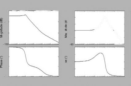
With the values given obtain the missile TF, its characteristic modes, frequency responses, and step input responses.

Solution

The following TF is obtained:

ay(s) 197s2 + 569.33s – 467(1463.16 – 60.87)

Й(?Г _ s2 + 5.63s + (7.92 + 144.3)

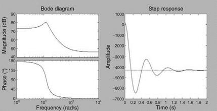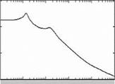
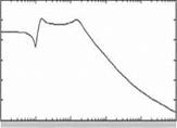
The latex dynamic mode is second-order oscillatory: -2.815 ± 12.0123i; the natural frequency is 12.3 rad/s; and the damping ratio is 0.228. The frequency response and the unit step rudder response for the latex are shown in Figure 5.9.

One of the real roots with a small value (relatively long time-period) indicates the spiral mode. The root can have a negative or positive value, making the mode convergent or divergent. This mode is dominated by rolling and yawing motions; sideslip is almost nonexistent. The characteristic root l for spiral mode is given by

LpNr — LrNp l

Lb

DR Frequency and Damping Ratio

1.08 rad/s 0.328

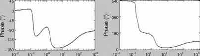
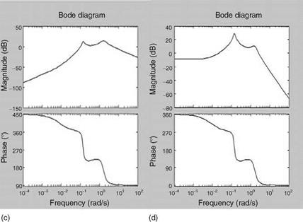
(c) (d)

FIGURE 5.7 DR mode frequency responses of a fighter aircraft. (a) Beta/aileron, (b) yaw rate/aileron, (c) beta/rudder, and (d) yaw rate/rudder.

Increasing Lb (dihedral effect) or Nr (yaw damping) will make the spiral mode more stable.

5.4.3 Roll Mode

(c) (d)

l = Lp (5.30)

Here, Lp is the roll damping derivative.

Roll subsidence mode is a first-order convergent mode of relatively short time constant.

In summary, DR is the dominant characteristic of any aircraft. However, its dominance in the roll angle TF is very small. This is because a quadratic numerator in the roll, aileron TF, almost cancels the DR denominator. Thus, the DR excited by the aileron is more predominant in roll rate and AOSS. The rudder contribution to the roll rate is small. The DR damping is usually positive, referring to Equation 5.28.

Therefore, the 2DOF DR mode would be a damped oscillation, or worst case divergence/subsidence. The 3DOF DR approximation would incorporate roll rate as an additional state variable. This will then have three roots: the spiral mode, the roll subsidence mode, and DR. The 3DOF spiral and roll subsidence approximation can also be made. The roll subsidence mode is dominant in the rolling motion. In the spiral mode the rolling and yawing motions predominate. Mostly unstable, the mode has a very large time constant. It is a fairly coordinated rolling and yawing motion mode.

and assuming no control inputs, the simplified form of a state-space model for the DR oscillatory mode can be expressed as [2]

Solving for the eigenvalues of the characteristic equation yields the following expressions for the natural frequency and damping ratio for this oscillatory mode:

Example 5.6

The state-space model of the DR mode of a supersonic fighter aircraft is given as

With the derivatives incorporated into this model we obtain

-0.139 2.218/75- 1.125 -0.571

Solution

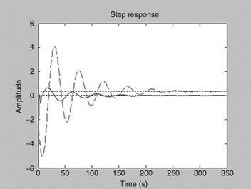
Following the procedure outlined in previous examples, four TFs are obtained (Table 5.4). The frequency responses are shown in Figure 5.7. The unit step responses for sideslip and yaw rate are shown in Figure 5.8; the lightness of the damping is evident from these responses.

Going back to the nonlinear coupled differential equations defined in Equations 3.22, 3.23, and 3.28, the general free lateral-directional motion of an aircraft can be described by eliminating the V, a, q, and U equations from the 6DOF state model. This leaves us with the following set of differential equations:

g

b = — (cos b sin f cos U + sin b cos a sin U — sin a cos f cos U sin b)

+ p sin a — r cos a + Щ – Cywind + —- cos (a + sj) sin b mV mV

t> = j jX_j 2 {qSb(IzCi + IxzCn) — qr(llz + I2 — Iylz) + pqlxz {lx — Iy + fz)}

lXlZ Lxz

r = X 2 {qSb(IxCn + IxzCi) — qrIxz{lx — Iy + Iz) + pq{llz + Il — IxIy)}

jxjz xz

f = p + q tan U sin f + r tan U cos f

ф = r cos f sec U + q sin f sec U (5.23)

These equations and the a, q, and U equations in Equation 5.6 make it clear that having a pure lateral-directional motion, in the strict sense, is unrealistic. However, if the excursions are small, it may not be totally wrong to neglect the longitudinal motion altogether. Also, from Equation 3.30, we have

Cywind = Cycos b + Cd sin b

For small values of b, we obtain

CYwind

Since the variable ф does not appear in any of the equations for b, p, r, and f, the ф equation is generally omitted from the analysis. Using the above assumptions in b equation, a simplified set to describe the lateral-directional motion can be written as

One can find several approximate forms of the EOMs in the literature [1-4]. The above form of the lateral-directional EOMs, expressed using nondimensional force and moment coefficients, is of more general nature. Further, the coefficients CY, Cl, and Cn can be expressed in terms of stability and control derivatives using Taylor series expansion as discussed in Chapter 4.

Expressing the side force, rolling, and yawing moments in terms of dimensional derivatives, the following state-space model can be used to describe aircraft lateral – directional motion for most applications:

where u0 and 00 are the forward speed and pitch angle, respectively, under steady – state condition.

The above state model can be used to obtain the lateral-directional characteristic equation. Solving it for the eigenvalues will yield two real roots corresponding to the spiral mode and roll subsidence, while a pair of complex roots defines the Dutch roll (DR) mode. These three distinct lateral-directional modes are briefly discussed here.

Example 5.5

The Douglas DC-8 aircraft state-space lateral-directional model [4] is given as

Obtain all the eight TFs using MATLAB. Obtain the characteristic modes of the aircraft dynamics.

Solution

The TFs are obtained by [numail, denail] = js2t/(a, b,c, d,1); [numrud, denrud] = ss2t/(a, b,c, d,2). For aileron input:

sysva = t/(numail(1,:),denail); syspa = t/(numail(2,:),denail); sysr = t/(numail(3,:), denail); and dampsystpha = t/(numail(4,:),denail).

For rudder input: sysvrud = t/(numrud(1,:),denrud); sysprud = t/(numrud(2,:),den – rud); sysrrud = t/(numrud(3,:),denrud); and systphrud = t/(numrud(4,:),denrud). These TFs are given in Table 5.2.

In fact this shows the feasibility of separately representing these modes in three different characteristic modes, since these modes seem to be reasonably well separated (Table 5.3).

The phugoid mode is a lightly damped low-frequency oscillation. The aircraft responses in phugoid are very slow compared to the changes in the motion parameters in SP mode. Chapter 7 shows a time history plot for the phugoid mode. This mode describes the long-term translatory motions of the vehicle center of mass with prac­tically no change in the angle of attack. This mode involves fairly large oscillatory changes in forward speed, pitch angle U, and altitude h at constant angle of attack.

An approximation to phugoid mode can be made by omitting the pitching moment equation:

(5.20)

where g is the acceleration due to gravity.

Forming the characteristic equation and solving for the eigenvalues yields the following expressions for the phugoid natural frequency and damping ratio:

Xu

2wnph

Example 5.4

The aerodynamic derivatives of a transport aircraft in phugoid mode are given as Xu — —0.015, Zu — —0.1, u0 — 60 m/s

Use the phugoid model of Equation 5.20 and obtain the frequency responses and other characteristics.

Solution

The state-space model is written as

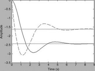
Based on the procedure of the previous examples, the TFs and the frequency responses are obtained for this phugoid model. The natural frequency of this mode is 0.128 rad/s and the damping ratio is 0.0587. The frequency and unit step responses are shown in Figure 5.6. Since the damping ratio of this mode is very small, the oscillations last for several seconds. Since the amplitudes are small and oscillations are of low frequency, the pilot would be able to manage these oscillations very well.

There is a possibility of a 3DOF phugoid approximation model. This can be done by retaining the derivatives related to the vertical speed:

(s — Xu)u — Xww + gU — XSe Se —Zuu + (s — Zw) w — Uos6 — ZSe8e —Muu — Mww — MSe 8e

With

Generally the phugoid frequency and damping increase in proportion to Mu.

In summary, we see that free longitudinal motions of the aircraft comprise of two oscillatory mode characteristics. This means that the forward velocity to elevator amplitude/magnitude (of the TF) will be much smaller at the natural frequency of the SP compared to that at the phugoid frequency. The phugoid mode will not have any change in the angle of attack. The higher vertical acceleration has a pronounced effect on the altitude and its rate of change. In general, irrespective of the size and weight of an aircraft, its basic characteristics can be described in a very simple manner in terms of only a few parameters, say two or four aerodynamic derivatives. This is made possible because a linear system is applicable to simplified dynamics and the related TF/control system concepts.

Bode diagram
0
-20 TS
-40
(a)
(b)

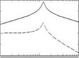
The SP is a relatively well-damped, high-frequency oscillation mode. Chapter 7 shows some typical time history plots of longitudinal SP motion. The amplitude ratio

Since a « w, Equation 5.14 can also be written in terms of a instead of w:

a= – a + f1 + Zq)q + Zde 8e u0 u0 u0

q = Maa + Mqq + Mde 8e

Z

Zw = —; Mw

uo

Putting the SP two degrees of freedom model in state-space form x = Ax + Bu and neglecting Zq

The characteristic equation of the form (AI – A) for the above system will be

A2 — (m9 + —)a + (/MqZa — мЛ = 0 (5.17)

uo uo

Solving for the eigenvalues of the characteristic equation yields the following frequency and damping ratio for the SP mode:

Example 5.2

The aerodynamic derivatives determined from flight test conducted with 3-2-1-1 pilot stick command input for a transport aircraft are given as

Zq = -0.0085, Za = -0.480, Zq = Q.1Q2, ZSe = 0.652,

MQ = 0.472, Ma = -4.916, Mq = -1.946, Mde = -7.011

The Z-force derivatives are assumed to be normalized with longitudinal velocity component uQ.

Write an appropriate mathematical model and obtain TF and frequency response of the SP model.

Solution

Based on the derivatives given we can build the following longitudinal SP model:

a = Zq + Zaa + (1 + Zq)q + Zge 8,

q = M0 + Maa + Mqq + M8e 8e

The state-space form is given as

The TFs are obtained as [numsp, densp] = ss2t/(a, b,c, d,1) and sysalpha = t/(numsp(1,:), densp) and sysq = t/(numsp(2,:),densp). The bias/‘‘nought’’ derivatives are ignored. The two TFs are

a(s) 0.652s – 6.457 d q(s) -7.011s – 6.585

d(sj = s2 + 2.428s + 6.355 ™ d(s) = s2 + 2.428s + 6.355

The SP frequency and damping ratio are obtained as: [spfreq, spzeta] = damp (sysalpha) = [2.521 rad/s, 0.4816]. The frequency/Bode diagrams are shown in Figure 5.3. Thus, we see the distinct SP mode, though for a different aircraft.

Example 5.3

The aerodynamic derivatives for an air force medium transport aircraft are given as

Za/U0 = -0.66, ZSe/щ = 0.01, Ma = -1.74, Mq = -0.67, MSe = -5.33

Write an appropriate mathematical model and obtain TFs and frequency responses of the SP model. Also, obtain the unit step responses.

Solution

Based on the derivatives given we can build the following longitudinal SP model:

a = (Za/u0)a + q + (ZSe/uq )8e q — Maa + Mqq + Mge 8e

The state-space form is given as

The TFs are obtained as [num, den] — ss2t/(a, b,c, d,1) and sysalpha — t/(num(1,:),den) and sysq — t/(num(2,:),den). The two TFs are

a(s) 0.01s – 5.323 , q(s) -5.33s – 3.535

and

Se(s) s2 + 1.33s + 2.182 8e(s) s2 + 1.22s + 2.182

The SP frequency and damping ratio are obtained as [spfreq, spzeta] — damp(sysalpha) — [1.48 rad/s, 0.45]. The frequency/Bode diagrams are shown in Figure 5.4. The unit step responses are shown in Figure 5.5.

Assuming that the aircraft does not perform maneuvers with large excursion, it is possible to characterize the aircraft response to pitch stick inputs by considering only the lift force, drag force, and pitching moment equations.

Equation 3.22 gives the Euler angles, Equation 3.23 gives the differential equa­tions for the angular rates, and Equation 3.27 gives the polar form for V, a, and b. Assuming the aircraft to be symmetric about the XZ plane, i. e., Ixy and Iyz are zero, the general free longitudinal motion can be described by eliminating the b, p, r, and ф equations from the 6DOF state model. This leaves us with the following set of differential equations:

q cos ф — r sin ф

In the above set, although the differential equations for b, p, r, and ф are omitted from analysis, these terms still appear on the right-hand side of the equations. Measured values of b, p, r, and ф can be used to solve the above equations. Equation

5.6 can be further simplified by assuming these quantities to be small during longitudinal maneuvers and neglecting them altogether. This gives the following set of equations:

V = g( cos U sin a — sin U cos a) — — CDwind H— cos (a + sT) cos b

mm

a = — (cos U cos a + sin U sin a) + q — ~qSCL——- sin (a + sT)

V mV mV

q = Y { qScCm + T(ltx sin St + ltz cos St)}

Iy

We also know from Equation 3.30 that

Cowind = Cd cos b — Cy sin b

For small values of b

CDwind — CD

aircraft dynamics has two distinct modes: one at lower frequency and another at relatively higher frequency. This shows the feasibility of modeling these two modes separately as they are relatively well separated. One can also discern from these plots that the low- frequency mode is lightly damped compared to the higher-frequency mode, which is confirmed in Table 5.1.

In fact this shows the feasibility of separately representing the modes in two different characteristic modes, since these modes seem to be well separated. We see from Figure 5.2 that the pitch rate response is well damped and the pitch attitude response takes more time to settle. This leads to the two distinct modes discussed in the next section.

In this approach, we do away with some of the differential equations from the state model and work with a reduced set of equations. However, since the eliminated variables will mostly appear in other equations, measured values of these variables from flight data are used. A very good example is that of the model equations used to analyze data generated from longitudinal short period (SP) maneuver. It is well known that during an SP pitch stick maneuver, there is only marginal change in velocity, implying that the longitudinal SP modes are more or less independent of velocity. Therefore, in the a, b, V form of equations, the V equation can be omitted from SP data analysis. Instead, the measured value of V can be used in the model equations without any loss of accuracy. The measured data for the variables used in this manner are sometimes referred to as ‘‘pseudo control inputs.’’

It is clear from the above discussion that the use of this approach would require measurements of the motion variables omitted from analysis. The disadvantage of this approach is that it is sensitive to the noise in the data.

Since most aircraft can be assumed to be symmetric about the XZ plane and fly at small sideslip angles, further simplification is possible by separating the 6DOF coupled equations into nearly independent sets: longitudinal and lateral-directional. Each set has nearly half the number of differential equations in the state model compared to the full coupled nonlinear 6DOF state equations. The simplified nondimensional and dimensional models normally used for longitudinal and lateral-directional flight data analysis are discussed next.