Our heavyweight helicopter equal in the world does not have
In Rostov started production of the most load-lifting rotary-wing car The Russian holding «Helicopt[...]

Everything about aircrafts and helicopters. News and events in aviation worldwide. Civil, transportation, military helicopters and airplanes.

Everything about aircrafts and helicopters. News and events in aviation worldwide. Civil, transportation, military helicopters and airplanes.

Everything about aircrafts and helicopters. News and events in aviation worldwide. Civil, transportation, military helicopters and airplanes.

Everything about aircrafts and helicopters. News and events in aviation worldwide. Civil, transportation, military helicopters and airplanes.


Unlike the fixed-wing aircraft, the lift propulsion and control in helicopters are provided by the main rotor (Figure 3.14). Helicopters have the ability to take off vertically, hover, and land even on unprepared terrain. In a helicopter, the upward lift is obtained by keeping the rotor shaft vertical. The main rotor system of the helicopter should be regarded as a lift-generating mechanism like the wings of an aircraft. The rotors/airfoils produce the lift. The rotor system could be semirigid, rigid, or fully articulated. The engine provides the power to the main rotor and the tail rotor. In a fully articulated rotor, each blade can rotate about the pitch axis that is feathering. This rotation changes the angle of attack and hence the lift. The blade can
move back and forth, that is, lead/lag movement. The blade can also flap up and down. Generally, such a system is used for helicopters with more than two blades. A semirigid rotor has two blades, and when one blade flaps up, the other blade will flap down. There is no lead/lag in this system. The rigid rotor does not provide lead/lag or flapping. Some of this is achieved by the blending of the blades.
Helicopters are inherently unstable and hence small movements of the control inputs are required.
Pedals: Pedals in helicopter are like those in an aircraft, and they can be operated to change the pitch in the tail rotor. The tail rotor is used to counteract the torque effects on the airframe by the main rotor. The pedals are not used to coordinate the turn. The pedals are used to trim the aircraft. The right and left pedals are for yawing to the right and left, respectively.
Collective and throttle: The collective lever increases the pitch in the main rotor collectively. You can raise the collective in the hover condition to gain altitude. The throttle also rotates backward. The collective control thus enables the power change and vertical motion. It controls the pitch of all the blades of the rotor collectively.
Cyclic: This is used for changing the position in hover or forward flight. If the rotor disk is tilted forward with the cyclic control, the outcome is a forward motion. If the cyclic stick is pulled backward, rearward motion is generated. Thus, the cyclic stick enables turn maneuvers and forward movements. It also provides for change in roll and pitch attitude.
To achieve forward or backward motion, the shaft is tilted in the desirable direction. To maneuver, the rotor plane is tilted relative to the horizontal plane to generate the necessary moments. During descent, the flow on the main rotor is reversed and lift is produced even when the engine is turned off. This phenomenon of autorotation can be used to make landings with a failed engine. To fly a helicopter, four types of controls are used. The vertical control is achieved by increasing or
decreasing the pitch angle of the rotor blades. This increases or reduces the thrust, thus changing the altitude of the helicopter. In a single main rotor helicopter, by changing the thrust at the tail rotor, a yawing moment is created about the vertical axis, which is used to provide the directional control. The longitudinal and lateral controls are applied by tilting the main rotor thrust vector. The helicopter would also employ autopilots, fly-by-wire controls, and couple controls.
When talking about rotorcraft dynamics, it is necessary to mention the momentum theory and the blade-element theory. While the momentum theory provides a basic understanding of the flow through the main rotor and the power required to produce thrust to lift the helicopter, it cannot be used alone to design the rotor blades. The blade-element theory looks into the details of how the thrust is produced by the rotating blades and relates the rotor performance to design parameters. The momentum theory for a rotorcraft in hovering condition is discussed next.
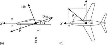
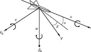
As in the case of aircraft, the axis system for missiles for the development of EOM is also assumed to be centered at the CG and fixed to the body. Figure 3.13 shows the X, Y, and Z axes, which are also the roll, pitch, and yaw axes, respectively. The XY plane represents the yaw plane while the XZ plane is the pitch plane. The angle of incidence in the XZ plane is a, the sideslip angle in the yaw plane is b, and the ay in Figure 3.12 denotes the flank angle. After a few simple algebraic calculations, the following relation can be easily obtained from Figure 3.13:
tan b = tan ay cos a (3.31)
 |
и, v, and w are the velocity components in the body axis. Compared to v and w, the component u is much larger and varies little during the flight. Like the aircraft, the missile too has 6DOF motion, which is represented by three forces and three moment equations [8]. The standard set of equations normally used to compute missile dynamics is similar to Equations 3.11 and 3.15
FIGURE 3.13
Fx = m(ii + qw — rv)
Fy = m(v + ru) (3.32)
Fz = m(W — qu)
L = pIx — qlxy — rlxz + qr(Iz — Iy) + (r2 — q2)Iyz — pqlxz + rpIxy M = – pixy + qly — rlyz + rp(Ix — Iz) + (p2 — r2)Ixz — qrIxy + pqlyz (3.33)
N = —pixz — qiyz + riz + pq(Iy — Ix) + (q2 — p2)Ixy — rpIyz + qrixz
The FX equation includes i, which represents the change in the forward speed. To
compute this, we need to know the drag force and the thrust force acting on the missile. Since w and v are generally small, the contribution of the terms pw and pv in equations for FY and FZ will be small if and only if the roll rate is small. From another perspective, the rolling motion will cause forces in pitch and yaw plane, a feature that is highly undesirable and should be dealt with at the design stage. The undesirable effects of high roll rate may also be reduced using acceleration feedback from autopilot during the flight.
If the roll rate p is assumed to be small and the flight variables q, r, v, and w being small, EOM for the missile can be simplified by neglecting the terms involving the products of these variables, e. g., terms like pv, pw, pq, and pr. In addition, assuming the missile to be reasonably symmetrical about the XZ and XY planes, the simplified set of equations can be written as
Fx = m(u + qw — rv)
![]() Fy = m(v + ru)
Fy = m(v + ru)
Fz = m(w — qu)
L = p Ix
![]() M = qIy
M = qIy
N = rIz
The rolling moment equation here shows no coupling between the roll and pitch motions and the roll and yaw motions.
At times, it is useful to work with equations expressed in polar coordinates for the following reasons:
• It is more convenient to use equations in polar coordinate terms as the aerodynamic forces and moments are easier to visualize and express in terms of angle of attack a, sideslip angle b, and velocity V.
• Flow angles a and b can be directly measured, and hence yield simple observation equations.
• Primary disadvantage, however, is that the system becomes singular at zero velocity, for the hover condition of a rotorcraft. Also, singularity occurs at beta equal to 90°.
V, a, and b in terms of u, v, and w are given by the following expressions (Figure 3.11):
![]() _1 w a = tan — u
_1 w a = tan — u
b = sin-1 V
Differentiating the above equations, we get
![]()
|
|
|
|
|
|
|
|
|
|
|
|
|
![]()
|
|||
|
|
||
|
|||
|
|||
|
|||
|
|||
|
|||
|
|||
|
|||
|
|||
Any of the above forms (rectangular or polar) can be used to describe the aircraft motion in flight. Note that there are no small angle approximations used, but equations have singularity at U = 90°. Further, there are several trigonometric and kinematic nonlinearities in the 6DOF equations.
Analysis of the full 6DOF equations would require a nonlinear program. The 6DOF model postulate is useful where nonlinear effects are important and coupling between the longitudinal and lateral modes is strong.
Although it is possible to analyze the 6DOF models, it is always a good idea to work with simplified models. These will be discussed in Chapter 5.
Using Equation 3.11 and Equations 3.15 through 3.19, the following nine coupled differential equations describe the aircraft motion in flight.
Force equations:
m(u + qw — rv) — qSCx — mg sin U + T cos sT
m(v + ru — pw) — qSCy + mg sin f cos U (3.20)
m(w + pv — qu) — qSCZ + mg cos f cos U — T sin sT
Moment equations:
qSbCi — p Ix — q Ixy — r/xz + qr(/z — Zy) + (r2 — q2)/yz — pq/xz + rp/xy qScCm — —_/xy + <q/y — r/yz + rp(/x — Iz) + (p2 — r2)/xz — qr/xy + pq/yz (3.21)
qSbC„ — —_ /xz — ^/yz + Г/z + pq(/y — /x) + (q2 — p2)/xy — rp/yz + qr/xz
Euler angles and body angular velocities:
f — p + q tan U sin f + r tan U cos f U — q cos f — r sin f (3.22)
fi — r cos f sec U + q sin f sec U
The above set of equations represents the 6DOF motion of the aircraft in flight. These can rearranged and expressed in two equivalent forms of equations.
3.5.1 Rectangular Form
 |
|
When the velocity is represented in a rectangular coordinate system, Equations 3.20 through 3.22 can be rearranged to yield the following set of equations in rectangular form:
p = l_ 2 {qSb(IzCi + IxO — qr(I2xz + l2 — Iylz) + pqlxzdx — Iy + Iz)} lxlz 1xz
q = J {qScCm — (p2 — r2)Ixz + pr(Iz — Ix) + T(itx sin St + itz cos St)} (3.23)
Iy
r = l_ 2 {qSb(IxCn + IxzCi) — qrIxz(Ix — Iy + Iz) + pq(12 + iI — Uy)}
IxIz — Ixz
f = p + q tan U sin f + r tan U cos f U = q cos f — r sin f C = r cos f sec U + q sin f sec U
Note that the terms in the rectangular boxes in the expressions for U, v, and w are the linear accelerations. This gives a set of kinematic equations, which can be used to check data consistency and estimate calibration errors in the data. The model equations normally used for kinematic consistency check are
U = —qw + rv — g sin U + ax v = —ru + pw + g cos U sin f + ay w = —pv + qu + g cos U cos f + az
f = p + q tan U sin f + r tan U cos f (3.24)
U = q cos f — r sin f C = r cos f sec U + q sin f sec U h = u sin U — v cos U sin f — w cos U cos f
The most significant contribution to the external forces and moments comes from aerodynamics. The three aerodynamic forces and moments in terms of nondimensional coefficients are
![]() Fxa — qSCx FyA — qSCy FzA — qSCz L — CiqSb M — CmqSc N — CnqSb
Fxa — qSCx FyA — qSCy FzA — qSCz L — CiqSb M — CmqSc N — CnqSb
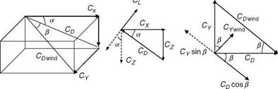
Here, the coefficients CX, CY, CZ, Q, Cm, and Cn are the nondimensional body axis force and moment coefficients; S represents the reference wing area; qc is the mean aerodynamic chord; b is the wingspan; and qq is the dynamic pressure. Further theory of aerodynamic coefficients is discussed in Chapter 4. In particular, the coefficients would be dependent on Mach number, flow angles, altitude, control surface deflections, and propulsion system. For example, a deflection of a control surface would mean an effective change of the camber of a wing. This will affect the lift, drag, and moments and hence the aerodynamic coefficients. In fact, these are ‘‘static’’ coefficients and are generally determined experimentally from various wind tunnel tests. Hundreds of such experiments are required to be done for various scaled-down models of the given aircraft. The aerodynamic effects during aircraft maneuvering flights are captured in aerodynamic derivatives (Chapter 4). Lift and drag are explained in Appendix A. Here, these aerodynamic coefficients [7] are described briefly to connect the EOM with aerodynamics. Typical values of these coefficients are given in Figure 3.8a and b.
Lift coefficient: This coefficient, CL, is related to Cz. Its contributions come from wings, fuselage, and horizontal tail. It varies with alpha and Mach number (Figure A4). An increase in drag is always associated with an increase in lift. If the camber of the wings is not much, then the lift is obtained from the higher dynamic pressure. Generally, in an aircraft there would be some mechanisms to increase the effective camber of the wings. These are the additional small surfaces like flaps, the deployment of which would provide the required lift at low dynamic pressures. The dependence of the lift coefficient on the angle of sideslip and altitude is usually
 |
|||
|
|||
|
|
![]()

small and hence negligible. However, the effect of the thrust and the Mach number on the lift coefficient would be significant. With higher thrust, the peak of the lift curve (the lift coefficient plotted vs. alpha) could increase and the peak could also shift to a higher angle of attack. The effect of Mach number is such that the slope of the curve would increase up to a certain Mach number and then start decreasing. For supersonic speeds, the peak would decrease. The relationship between CL, CN, and CZ is given in Appendix A and Equation (3.29); CN is the normal force coefficient.
Drag coefficient: This coefficient, CD (Figure A5), is related to Cy, CN, and Cx in general. The latter is called the axial force coefficient. This is an important design parameter for the aircraft. In an ideal situation, one would always like to have minimal drag, no resistance to the aircraft, and the maximum possible lift (so that the aircraft can carry very large loads). This intuitive requirement defines the lift/drag (L/D) ratio and it is a performance parameter. The drag force is not necessarily a linear combination of several components: friction drag, form drag, induced drag, and wave drag. The individual contributions of these effects on the total drag would change with the flight conditions.
Side force coefficient: This force is the result of the aircraft having a sideslip angle different from zero. In general, the sideslip force depends on alpha, beta, Mach number, rudder control surface deflection, roll rate, and yaw rate.
Pitching moment coefficient: This is a very important parameter for the stability of the aircraft, especially in its derivative form, i. e., Cm. The latter is supposed to be negative in general. However, when it is positive, the aircraft does not have the required static stability. This aspect is discussed in Chapter 4. If the slope of the moment curve is high, then the aircraft is said to have pitch ‘‘stiffness.’’ Thus, a trade-off is required between static stability and maneuverability. The reduced/ relaxed static stability airframes are specially designed to obtain high L/D ratio and good maneuverability. The statically unstable configurations for obtaining such benefits, however, need to be artificially stabilized by feedback control filters/ algorithms. The moment coefficient primarily depends on alpha, Mach number, altitude, pitch rate, elevator (or elevon for delta wing aircraft) control surface deflection, inertial damping, aerodynamic damping term Cma, and flap displacement.
Rolling moment and yawing moment coefficients: These coefficients depend primarily on alpha, beta, Mach number, roll rate, yaw rate, aileron control surface (or elevon for the delta wing configuration) displacement, and rudder control surface deflection. These coefficients are better understood in the form of their components, which are discussed in Chapter 4.
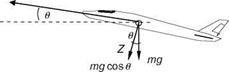
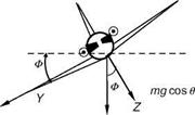
Next, to resolve the gravitational force acting on the aircraft into components along the body axis (Figure 3.9), the relative orientation of the gravity vector to the body axis system is required. If f, U, and C are the angular orientations of the gravity vector with respect to body x, y, and z axes, respectively, the components can be written as
FxG = – mg sin U
FyG = mg sin f cos U (3.17)
Fzg = mg cos f cos U
|
The third component comes from the engine thrust. Assuming the engine tilt angle to be sT with respect to the body X-axis and the total applied forces (accounting for the contribution from aerodynamic, gravity, and thrust) can be expressed as
Fx = qSCx — mg sin U + T cos sT
Fy = qSCy + mg sin f cos U (3.18)
Fz = qSCz + mg cos f cos U — T sin sT
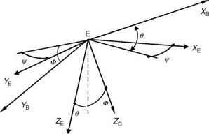
At times, contribution from the gyroscopic moment from the propulsive system is added to the moment equations. This contribution is, however, neglected in the present model postulates. Although the forces and moments expressed here have been derived for the body axis frame of reference, the orientation of the aircraft has to be described with respect to a fixed reference frame. Assuming the body axis and the fixed frame to be parallel, three angular rotations in the following specific order are applied to determine the Euler angles (Figure 3.10):
• Rotate the fixed frame through yaw angle C to attain frame position x1,
y1, z1.
• Rotate x1, y1, z1 frame through pitch angle U to attain the position x2, y2, z2.
• Rotate x2, y2, z2 frame through roll angle f to attain the position x3, y3, z3.
The frame x3, y3, z3 is the final orientation of the body axis to the fixed axis. The relationship between the body axis angular rates p, q, and r and the Euler rates C, U, and f, derived from Figure 3.9, can be expressed as
f = p + q tan U sin f + r tan U cos f U = q cos f — r sin f (3.19)
C = r cos f sec U + q sin f sec U
Example 3.3
Express the inertial velocity components x, y, Z in terms of the velocity components u, v, w in body axis.
In Figure 3.10, rotation of the frame through ф to position xb y1, zi gives
x — u1 cos ф — v1 sin ф y — u1 sin ф + v1 cos ф Z — w1 (because rotation is about z-axis)
Next rotation through U to position x2, y2, z2 gives
u1 — u2 cos U + w2 sin U v1 — v2 (because rotation is about yj-axis) w1 — w2 cos U — u2 sin U
Final rotation through f to position x3, y3, z3 gives
u2 — u (because rotation is about yj – axis) v2 — v cos f — w sin f w2 — v sin f + w cos f
Substituting u2, v2, w2 by ub vi, wi, we obtain
ui — u cos U + [v sin f + w cos f ] sin U v1 — v cos f — w sin f w1 — [v sin f + w cos f ] cos U — u sin U
Substituting u1, v1, w1 by X, y, Z, we obtain
X — [u cos U + (v sin f + w cos f) sin U] cos c — [v cos f — w sin f ] sin c y — [u cos U + (v sin f + w cos f) sin U] sin c + [v cos f — w sin f ] cos c Z — [v sin f + w cos f ] cos U — u sin U
In the matrix form
|
x |
cos U cos c sin U sin f cos c — cos f sin c sin U cos f cos c + sin f sin c |
u |
|
|
y |
— |
cos U sin c sin U sin f sin c + cos f cos c sin U cos f sin c — sin f cos c |
v |
|
z_ |
— sin U cos U sin f cos U cos f |
w |
|
Note that the matrix is the same as the transformation matrix given in Equation A.34. |
The right-hand side of Equation 3.8 contains the term V, which represents the time derivative of velocity with respect to the body axis system. The cross product terms (v x V) arise from the centripetal acceleration along any given axis due to angular velocities about the remaining two axes. In component form we have
V = ui + vj + wj
v = pi + qj + rj (3.10)
H = Hxj + Hyj + Hzj
Using the above expressions in Equation 3.8, we have
F = m [[Ui + vj + Wj] + (pi + qj + rj) x (ui + vj + wj)]]
F = m[U + qw — rv]i + m[v + ru — pw] j + m[W + pv — qu]k
Thus, the force components acting along the X, Y, and Z body axes are
Fx = m(u + qw — rv)
Fy = m(v + ru — pw) (3.11)
Fz = m(w + pv — qu)
Example 3.1
Assume two-dimensional accelerated flight of an aircraft. In this situation U + DU and V + Д V would have rotated by an incremental angle R Dt. Of course, the aircraft would also have rotated through the same angle. Here U and V are the total velocities of the aircraft in forward and lateral directions. Then the equation for the rectilinear longitudinal acceleration can be easily derived.
,• ,* ™(U + DU)cos(R Dt) — U — (V + Д V) sin(R Dt)
aX = lim(Dt! 0)—————————- d—————————-
Since the limit of sin(RtDt) = R, we finally obtain for small changes/perturbation
aX = U_ — VR
Example 3.2
Assume two-dimensional accelerated flight of an aircraft. Derive the equation for the corresponding rectilinear lateral acceleration.
We have for this case the following formula:
, (U + DU) sin(R At) + (V + DV) cos(R At) – V
ay = lim(At! 0)————————- A—————————–
Using the same reasoning as the previous case, we get
ay = V + UR
Such small perturbation terms appear in Equation 3.11 as can be clearly seen.
From Equation 3.9, we have
M = H + (v x H)
The total moment about a given axis is due to both direct angular acceleration about that axis and those arising from linear acceleration gradients due to combined rotations about all axes. The components of angular momentum about the three axes are given by
Hx = pix q1xy r1xz
Hy = – pixy + qly – rlyz (3.12)
Hz = pizx qizy A riz
Even though there could be variation in the mass and its distribution during a flight due to fuel consumption, use of external stores, etc., the assumption that the mass and mass distribution of the air vehicle are constant is reasonable and simplifies the expression for the rate of change of angular momentum. The time derivatives of the angular momentum components expressed in body axis are given by
Hx = pix – q ixy – rixz
Hy = – pixy + qiy – riyz (3.13)
Hz pizx qizy A riz
To get the total time rate of change of angular momentum, and thus the scalar components of the moments, we must add to these contributions arising because of steady rotations (v x H).
L = Hx – rHy + qHz
M = rHx + Hy – pHz (3.14)
N = —qHx + pHy + Hz
Substituting for angular momentum components and regrouping results, the moment equations can now be written (with respect to the body axis system) as
L — plx qIxy rIxz T qr(Iz Iy) F (r q )Iyz pqIxz F rplxy
M — – pixy + qIy – rIyz + rp(Ix – /z) + (p2 – r2)/xz – qrIxy + pqlyz (3.15)
N pIxz qIyz F rIz F pq(Iy Ix) T (q p )Ixy rpIyz T qrIxz
The total forces and moments acting on the aircraft are made up of contributions from the aerodynamic, gravitational, and aircraft thrust.
When describing aircraft flight path, it is necessary to mention the reference axis system of the aircraft and its relation to the Earth. Thus, a proper understanding of the various axes systems and their transformation is of importance. The frequently used axes systems are the inertial, Earth, body, wind, and stability axes and their definitions are as follows.
 |
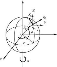
Inertial axis: The origin of inertial axis system is assumed to be the center of the Earth. This reference frame is assumed to be stationary with the z-axis pointing to
|
z
FIGURE 3.3 Inertial axis system. (From Chetty, S. and Madhuranath, P. (ed.), Aircraft Flight Control and Simulation, NAL Special Publication 9717, FMCD, NAL, 1998.) |
the North Pole and the x-axis pointing to 0° longitude (Figure 3.3). The y-axis, perpendicular to the XZ plane, completes the right-handed orthogonal axis system.
Earth axis: The origin of the Earth axis system lies on the surface of the Earth, with the X – and Y-axes pointing to the north and east directions (NED). The z-axis points down toward the center of the Earth. This reference frame is fixed to the Earth and, at times, is referred to as the NED frame (Figure 3.4). For most aircraft modeling and simulation problems, it is assumed to be the inertial frame of reference where Newton’s laws are valid.
Body axis: The origin of the body axis system is fixed to the aircraft’s CG, and therefore rotates and moves in space along with the aircraft. The X-axis points forward through the aircraft’s nose and is called the longitudinal axis, while the positive
|
|
|
FIGURE 3.5 Body axis system. |
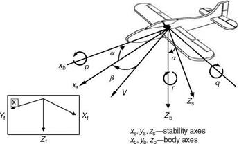
direction of the Y-axis is along the right wing and is known as the lateral axis. Thus, the X – and Y-axes are aligned with some geometric features of the aircraft. The Z-axis is perpendicular to the XY plane and points toward the Earth when the aircraft is in straight and level flight (Figure 3.5). In an alternative principal body axis, the X-axis is aligned with the principal inertia axis. Thus, the cross product of inertia, Izx, is zero. This would simplify the lateral EOM. Interestingly, the aerodynamic body axis (also known as stability axis in the United States and wind axis in the United Kingdom) has the X-axis aligned with the projection of the velocity vector, in a datum flight condition, onto the plane of symmetry. The aerodynamic body axis is at an angle a relative to the geometric body axis. Since, these axes are ‘‘natural’’ axes systems, they are used to define the basic aerodynamic forces, lift, and drag. The body axis angular rates and Euler angles are naturally measured quantities. This system is consistent in the use of the force coefficients in the body axis. However, it yields nonlinear observation equations for flow angles and velocity and also has singularity at a pitch angle of 90°. Interestingly, the pilot is aware of the rotations of the aircraft about its CG, rather than any other axis fixed in space. The pilot ‘‘feels’’ the accelerating movement of the aircraft because his alignment is in the body axis system.
Wind axis: The origin is at the aircraft’s CG with the X-axis pointing forward and aligned to the velocity vector. The positive Y-axis passes through the right wing and the Z-axis points downward. The aircraft flow angles (angle of attack and sideslip) define the relation between the wind and the body axis system (Figure 3.5). Since the direction of the aircraft velocity vector keeps changing during the flight, the wind axis system, unlike the body axis system, is not fixed.
Stability axis: This axis system is similar to that of body axis. The origin is at the aircraft’s CG and the Y stability axis is aligned with the Y body axis that passes through the right wing. The X stability axis is inclined to the X body axis at an angle AOA (Figure 3.6).
The aerodynamic data are generated in a wind tunnel in body axis or in stability axis. Thus, a clear understanding of the various axes systems used and the ability to transform from one to the other is essential to the study of aircraft dynamics. The axes systems are lined together by the direction cosine matrix, which is a function of the Euler angles f, U, C (Appendix A has more details on axis transformation).
|
|
|
Earth fixed
frame
As mentioned earlier, the core issue in flight mechanics is to evaluate the aircraft performance and dynamics. To evaluate aircraft performance indices such as range, rate of climb, takeoff, and landing distance, the aircraft is generally treated as a point mass model and its lift, drag, and thrust forces are identified. Although the point mass model is useful for a brief description of aircraft dynamics, the complete six-degree-of-freedom (6DOF) nonlinear equations would be required for a detailed description of aircraft dynamics. In between these two extremes lie the linearized models, which are useful for control design applications (Figure 3.7).
 |
Expecting the aircraft to behave like a dynamic system in flight, an input given by the pilot will cause the forces and moments acting on the aircraft to interact with its inherent natural characteristics, thereby generating responses. These responses
contain the natural dynamic behavior of the aircraft, which can be described by a set of equations called EOM with certain important assumptions.
1. Aircraft is a rigid body. This assumption, though strictly not valid, is sufficiently accurate for describing aircraft motion in flight. It allows the aircraft motion to be described by the translation of and the rotation about its CG. In reality, various components of an aircraft might move in relation to each other: engine, rotorcraft disk, control devices, and bending of wings (this brings aspects of aeroelasticity into flight dynamics problems) due to air loads.
2. Earth axis system can be used as the inertial frame of reference in which Newton’s laws are valid, and the Earth is assumed to be fixed in space.
3. Aircraft mass is constant. Though not always true, the mass distribution of the aircraft is assumed to be invariant.
4. Earth is flat for the period of time of dynamic analysis. The curvature effects would have to be taken into account only for long-range flights (e. g., missiles, spacecrafts, etc.).
5. XZ plane in aircraft is a plane of symmetry.
6. Steady flight is assumed to be undisturbed. This will simplify several equations, according to the needs of the case. If flow angles are assumed to be small, then sine and cosine terms would be simplified. This would render the applicability of the EOMs to the conditions where small perturbations could occur.
These basic assumptions are appropriately used in formulating the EOMs and their simplification as the case might be.
The EOM of the aircraft can be written by considering its linear and angular momentums.
Let p be the linear momentum vector (mV) and H the angular momentum vector, each measured in the inertial reference frame. Newton’s second law states that the summation of all the external forces acting on a body is equal to the time rate of change of momentum of the body:
![]() dp = d(mv) = v F dt ~ dt ~ ^
dp = d(mv) = v F dt ~ dt ~ ^
Similarly, the summation of all external moments acting on the body is equal to the time rate of change of the angular momentum (moment of momentum):
Referring to the inertia and angular velocities in the space fixed inertial frame, the inertia tensor will change as the aircraft rotates about the axes. This would contribute to dH/dt through dl/dt and the resulting equations would have time variant parameters. To overcome this, we consider the body axis system that is fixed to the aircraft so that the rotary inertial properties are constant. This implies that the vector quantities V and H in Equations 3.1 and 3.2 need to be determined in the body axis.
A vector in a body axis frame, rotating at an angular speed of ш, can be represented by the following equation:
Here, subscripts І and B refer to the inertial and body axes frame of references. Using the above expression, the forces and moments in the inertial axis system can now be represented in the body axis system as follows:
It must be emphasized here that the mass is assumed to be constant. This would not be the case for long-range aircraft flights, missiles, and spacecrafts because of expending of fuels/shedding away certain extended components/stages, etc.
The inertial forces and moments can now be resolved in the body axis system.
3.1 INTRODUCTION
In Chapter 2, a system was defined as a set of components or activities that interact to achieve a desired task. The primary requirement to study a system, be it a chemical plant or a flight vehicle, is a model that closely resembles the system. In other words, a model is a simplified representation of a system that helps to understand, predict, and possibly control its behavior. It presents a workable knowledge of the system and simulates its behavior. Some authors also refer to a model as a less complex form of reality.
A flight vehicle is a complex system that requires a number of models for its various components (Figure 3.1). In this chapter, we describe the model form that represents aircraft dynamics. When an aircraft flies, it experiences gravitational, propulsive, and inertial forces arising from the airflow over the aircraft frame. To achieve a steady, unaccelerated flight, these forces must balance out one another. The upward force, due to the lift, should be in equilibrium with the downward force, due to the weight of the aircraft, so that it does not experience unsteadiness (unintentional one). Similarly, the forward thrust force should be in equilibrium with the opposing drag force so that the aircraft does not accelerate and, hence, is steady. An aircraft satisfying these requirements is said to be in a state of equilibrium or flying at trim condition. Normally at trim, the translational and angular accelerations are zero. The notations and terms used in describing aircraft dynamics are given in Appendix A.
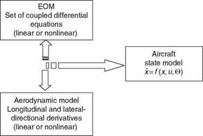
Both the equations of motion (EOM) and the models of the aerodynamic force and moment coefficients have to be postulated to describe the aircraft motion in flight (Figure 3.2). Aircraft EOM comprise aircraft motion variables (aircraft states) such as airspeed, flow angles (angle of attack and sideslip angles), angular velocities (pitch, rate, and yaw), and attitude angles (bank, pitch, and heading), formulated as differential equations. The collection of these aircraft motion variables is called the state vector, which helps describe the motion of the flight vehicle at any given point of time. Aircraft EOM are described in various textbooks and reports [1-6]. The core issue in flight mechanics is to evaluate aircraft performance and dynamics. The laws that govern the motion of an aircraft are those of Newton, provided the aircraft is a rigid body. It is well known that, at high velocities, aircraft dynamics are affected by structural elasticity. However, for understanding the dynamics of flight, it is convenient to consider aircraft as a rigid body with its mass concentrated at its center of gravity (CG). There are ways of adding on the aeroelastic effects to the rigid formulation. With this all-important assumption of the aircraft as a rigid body, we can elaborate on the forces and moments experienced by aircraft in flight, which we referred to in the definition of equilibrium of aircraft flight.
|
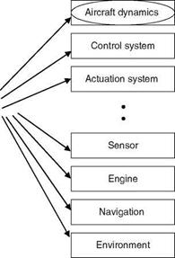
FIGURE 3.1 Aircraft model components.
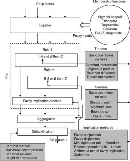
Each input partially fires all rules in parallel and the system acts as an associative processor as it computes the output F(x). The system then combines the partially fired ‘‘then’’ part fuzzy sets in a sum and converts this sum to a scalar or vector output. Thus, a match-and-sum fuzzy approximation can be viewed as a generalized AI expert system or as a (neural-like) fuzzy associative memory. Adaptive fuzzy systems (AFSs) have proven universal approximators for rules, which use fuzzy sets of any shape and are computationally simple. A feedback fuzzy system (rules feedback to one another and to themselves) can model a dynamic system: dx/dt = F(x). The core of every fuzzy controller is the fuzzy inference engine (FIE), the computation mechanism with which decisions can be inferred even though the knowledge may be incomplete. This mechanism gives the linguistic controller the power to reason by being able to extrapolate knowledge and search for rules, which only partially fit any given situation for which a rule does not exist. The FIE performs an exhaustive search of the rules in the knowledge base (rule base) to determine the degree of fit for each rule for a given set of causes (see Figure 2.19). The input and output are crisp variables.
Several rules contribute in varying degrees to the final result. A degree of fit of unit implies that only one rule has fired and only one rule contributes to the final decision; a degree of fit of zero implies that none of the rules contribute to the final decision. The knowledge necessary to control a plant is usually expressed as a set of linguistic rules of the form: If (cause) ‘‘then’’ (effect). These are the rules with
which new operators are trained to control a plant and they constitute the knowledge base of the system. All the rules necessary to control a plant might not be elicited or known. It is therefore essential to use some technique capable of inferring the control action from available rules. FL base control has several merits: (1) for a complex system, a mathematical model is hard to obtain, (2) fuzzy control is a model-free approach, (3) human experts can provide linguistic descriptions about the system and control instructions, (4) fuzzy controllers provide a systematic method to incorporate the knowledge of human experts. The assumptions in an FL control system are as follows: (1) the plant is observable and controllable, (2) expert linguistic rules are available or formulated based on engineering common sense, intuition, or an analytical model, (3) a solution exists, (4) one can look for a good enough solution (approximate reasoning in the sense of probably approximately correct solution, e. g., algorithm) and not necessarily the optimum one, and (5) one can desire to design a controller to the best of our knowledge and within an acceptable precision range. Figure 2.20 depicts a macrolevel computational schematic of the fuzzy inference process: fuzzification (using membership functions), basic operations (on the defined rules), fuzzy implication process (using implication methods), aggregation, and finally defuzzification (using defuzzification methods) [23,24]. Example 2.13 illustrates the definition of fuzzy membership functions (GMF, TMF, etc.) as seen in Figure 2.21, definition of fuzzy operators, numerical computations to obtain the fuzzy counterpart of the classical intersection and union, and comparison with other such operations. The example requires careful study, but tells us many simple things about fuzzy operators, which are routinely used in modeling and control of dynamic systems. In Chapter 9, we present an FL-based Kalman filter for aircraft state – estimation, whereby other aspects of fuzzy operations would be clear.
Example 2.13
The fuzzy operators corresponding to the well-known Boolean operators AND and OR
are, respectively, defined as min and max [23,24]:
![]()
 |
mAnB(u) = mm[mA(u), mB(u)] (intersection)
mAus(“) = max[mA(u), ^b(“)] (union)
|
FIGURE 2.20 Fuzzy inference system with implication process. |
Another method to define AND and OR operators has been proposed by Zadeh [23,24]:
mAns(u) = mA(u)mB(u) (7)
mAus(u) = mA(u) + тв(и) – mA(u)mB(u) (2-38)
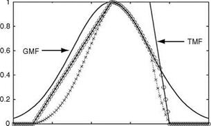
Define fuzzy sets A and B by Gaussian and Trapezoidal membership functions (see GMF, TMF in Figure 2.21) (mA(u), mB(u)), respectively. Obtain the fuzzy intersection (element wise) by placing mA(u) and mB(u) in Equations 2.35 or 2.37. In addition, obtain Fuzzy union (element wise) by using Equations 2.36 or 2.38.
|
0 2 4 6 8 10 |
|
(a) u—input variable
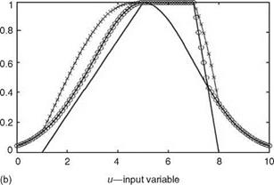
FIGURE 2.21 (a) Fuzzy intersection operations (Equation 2.37—x and Equation 2.35—O); (b) fuzzy union operations (Equation 2.38—x and Equation 2.36—O). |
Solution
The results are shown in Figure 2.21. Let us denote a — mA(u) and b — mB(u) to be membership grades (within interval [0,1]). Now assume that for some value of input u, a < b; therefore, mAnB(u) using Equation 2.35 will be
mAnB(u) = min (a, b) = a (2.39)
In addition, it is known that b < 1 and multiplying this expression with a gives ab < a. Using Equation 2.37 in the left hand side of ab < a results in ab < min(a, b) which shows that Equation 2.37 < Equation 2.35 (in the sense of the numerical values), i. e., the area covered by x-line (representing Equation 2.37) is lesser than that covered by 0-line (representing Equation 2.35). The same equality holds for a > b. The membership function obtained by Equation 2.38 expands compared to the one obtained by Equation 2.36 (Figure 2.21b). This can be easily proved by a numerical example. Let us assume a — 0.1 and b — 0.5 for some value of input variable u. By placing them in
Equations 2.38 and 2.36 we get тлив(и) equal to 0.55 and 0.5 (one can easily verify this), respectively, which means that Equation 2.38 > Equation 2.36, i. e., the area covered by x-line (representing Equation 2.38) is greater than that covered by 0-lines (representing Equation 2.36).
It is apparent from the above definitions that, unlike in crisp logic/set theory, the fuzzy operators can have seemingly different definitions. However, these would be mathematically consistent and would be intuitively valid and appealing [7].
EPILOGUE
Various models for representing dynamic systems have been considered in this chapter. The treatment has been kept as simple as possible. State-space and TF models are very appropriate for parameter estimation and system identification and also useful for evaluating the HQs of aircraft. ANNs and FL find several applications in control, simulation, and modeling [23,25,26]. In Ref. [27], the authors consider the application of NWs for assessing the behavior of the human pilot in the task of maintaining the flight path and airspeed during wind shear approaches. In Ref. [28], fuzzy modeling is proposed for identification, where data are classified by fuzzy clustering and then rules are extracted from these clusters.
The random phenomena that represent uncertainty are modeled by probability theory, which is based on crisp (binary) logic. Our interest is to model the uncertainty that abounds in nature and to discuss the need to model uncertainty in science and engineering problems. One way is to use crisp logic:
The crisp or Boolean characteristic function:
fA(x) = 1 if input x is in set A
= 0 if input x is not in set A
In classical set theory, a set consists of a finite/infinite number of elements that belong to some specified set called the universe of discourse. In crisp logic, we have answers like yes or no; 0 or 1; —1 or 1; off or on. Examples are (1) a person is in the room or not in the room, (2) an event A has occurred or not occurred, (3) light is on or off. However, real-life experiences indicate that some extension of crisp logic is definitely necessary. Events or occurrences leading to FL are (1) the light could be dim, (2) the day could be bright with a certain degree of brightness, (3) the day could be cloudy with a certain degree, and (4) the weather could be warm or cold. Thus, FL allows for a degree of uncertainty and gradation. Thus, truth and falsity (1 or 0) become the extremes of a continuous spectrum of uncertainty. This leads to multivalued logic and the fuzzy set theory [7]. Fuzziness is the theory of sets and a characteristic function is generalized to take an infinite number of values between 0 and 1: e. g., triangular form. Several types/forms of membership function are available in MATLAB FL toolbox.
Fuzzy systems can model any continuous function or system. The quality of approximation depends on the quality of rules that can be formed by experts. Fuzzy engineering is a function approximation (FA) with fuzzy systems. This approximation does not depend on words, cognitive theory, or linguistic paradigm. It rests on mathematics of FA and statistical learning theory (SLT). Much of the mathematics is well known, and as such there is no magic in fuzzy systems. A fuzzy system is a natural way to turn speech and measured action into functions that approximate hard tasks. Words are just a tool or a ladder we climb on to perform the task of FA. Fuzzy language is a means to the end of computing and not the goal. The basic unit of fuzzy FA is the ‘‘If then’’ rule: ‘‘If the wash water is dirty then add more detergent.’’ Thus, a fuzzy system is a set of ‘‘If then’’ rules, which maps input sets like ‘‘dirty wash water’’ to output sets like ‘‘more detergent.’’ Overlapping rules define polynomials/richer functions. A set of possible rules are given below [23]:
Rule 1: if the air is cold then set the motor speed to stop Rule 2: if the air is cool then set the motor speed to slow Rule 3: if the air is just right then set the motor speed to medium Rule 4: if the air is warm then set the motor speed to fast Rule 5: if the air is hot then set the motor speed to blast
This gives the first-cut fuzzy system. More rules can be guessed, formulated, and added by experts and by learning new rules adaptively from training data sets. ANNs can be used to learn the rules from the data. Much of fuzzy engineering deals with tuning these rules and adding new rules or pruning old rules.