Our heavyweight helicopter equal in the world does not have
In Rostov started production of the most load-lifting rotary-wing car The Russian holding «Helicopt[...]

Everything about aircrafts and helicopters. News and events in aviation worldwide. Civil, transportation, military helicopters and airplanes.

Everything about aircrafts and helicopters. News and events in aviation worldwide. Civil, transportation, military helicopters and airplanes.

Everything about aircrafts and helicopters. News and events in aviation worldwide. Civil, transportation, military helicopters and airplanes.

Everything about aircrafts and helicopters. News and events in aviation worldwide. Civil, transportation, military helicopters and airplanes.


Figure 4.4 shows a half-plan view of the example helicopter divided into segments by concentric circles around the rotor mast. Also shown is a side view with wake stations designated below the rotor. The drag coefficient for each segment depends on the shape of its cross section. Drag measurements of cylinders and flat plates under a rotor are reported in reference 4.1. It is concluded in that report that the turbulence in the rotor wake is always high enough to insure that fully turbulent, or supercritical, boundary-layer conditions exist. Supercritical drag coefficients for a number of two-dimensional shapes with flow from above are shown in Figure 4.5. These drag coefficients are based on data presented in references 4.1 and 4.2.
Tilt-rotor aircraft have a large wing to be accounted for. Deflecting a trailing edge flap can reduce its vertical drag penalty but wind tunnel test results reported in reference 4.3 indicate that the optimum flap angle is about 60° rather than the 90° that would be expected to produce less drag.
The measured distribution of dynamic pressure under a full-scale rotor with —4° of twist was shown on Figure 1.19 of Chapter 1. For rotors with different twist, the measured distribution can be modified by multiplying by the square of the ratio of induced velocities calculated by the method of Chapter 1 for the two values of twist. Figure 4.6 shows the —4° twist distributions modified for —10° of twist for use with the example helicopter.
Using the drag coefficients and the dynamic pressure corresponding to each of the airframe segments, the vertical drag penalty can now be calculated by
|
Radius Station, r/R |
Hemispherical Nose Cq = -1
Wheel CD = .25
— 7 Y / і I І і /
___ л і.
FIGURE 4.5 Drag Coefficients of Typical Component Shapes
Note: Drag coefficients are based on super critical flow and on area projected in plan view.
summing the product of the drag coefficient, the dynamic pressure ratio, and the projected area of each segment in the half-plan view:
N
D 2 X (^/D. L.)„A„
v_________ я^І__________________________
G. W Г A
Table 4-1 presents the calculation for the example helicopter, which shows that the download penalty is 4.2% of gross weight.
The saving in power due to the pseudo ground effect of the fuselage on the rotor may be estimated by calculating the ground effect due to a full ground plane at the mean position of the fuselage by the method of Chapter 1 and then multiplying it by the ratio of projected fuselage planform area in the wake to disc area. Thus:
|
—————- Extrapolated for Rotor with -10° Twist |
|
rlR FIGURE 4.6 Distribution of Dynamic Pressure in Wake |
Source: Boatwright, “Measurements of Velocity Components in the Wake of a Full-Scale Helicopter Rotor iri Hover,” USAAMRDLTR 72-33, 1972.
For the example helicopter the mean position of the fuselage is at Z/D = .12 and from Figure 1.41 of Chapter 1:
‘IGE
|
TABLE 4.1 Calculation off Vertical Drag for the Example Helicopter
|
For hovering at Cx/a = .086:
A Cq/o = -.00024
which is the equivalent of 68 horsepower.
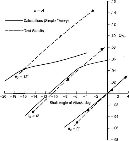
The method has been used to correlate with the test data reported in reference 4.4. These tests used a model helicopter suspended under a separate rotor. Both elements were mounted on individual balance systems and wings of various sizes and positions could be installed. Figure 4.7 shows the test results in terms of both vertical drag and pseudo ground effect (which corresponds to the "thrust recovery” of reference 4.4). Also shown are calculated values for the two quantities determined by – the foregoing method. It may be seen that in this case both the download and the pseudo ground effect calculations are optimistic for the fuselage alone, but for the fuselage with the large wing, the download is optimistic whereas the ground effect is pessimistic. Some of the discrepancy may be due to the relatively small size of the model and the possibility that some components actually experienced high drag, subcritical conditions in spite of the wake turbulence.
Measurements of vertical drag in ground effect are reported in reference 4.5 and are. summarized in Figure 4.8, which shows that both the vertical drag and the pseudo ground effect are reduced, or even reversed, when hovering less than a rotor diameter above the ground. Reference 4.6 reports that model tests on the Sikorsky S-76 show that the download ratio changes from +3% out of ground effect to —1% at a wheel height of one foot.
Losses which occur between the torquemeter and the rotors must be made up by the engine and are additive to the power required by the rotors. Sources of these losses include:
• Main rotor transmission
• Tail rotor gearboxes
• Engine nose gearboxes
• Transmission-mounted accessories such as generators and hydraulic pumps
• Cooling fans driven from the drive system
Gearbox and transmission losses are produced by friction between the gear teeth and in the bearings and by aerodynamic drag, or "windage.” The losses are a function of the size of the gearbox as well as the power being transmitted at any given time. For preliminary design purposes, the losses in gearboxes—including power to run their lubrication systems—can be estimated from the following equation:
•Power loss per stage = iC[Design max. power + Actual power], h. p.
where К = 0.0025 for spur or bevel gears and К = 0.00375 for planetary gears.
The example helicopter will be assumed to have two engine nose gearboxes with one stage of bevel gears, each designed for 2,000 h. p. The main rotor transmission has two spur gears stages and one planetary gear stage, with a design capacity of 4,000 h. p. The tail rotor drive system contains two gear boxes with one stage of bevel gears each and a design capability of 750 h. p. The total transmission losses are thus:
h-p-trans. = 0-0025 (4,000 + Eng. power) + 0.00875 (4,000 + Main rotor power)
+ 0.0050 (750 + Tail rotor power)
Assuming that the engine power is the sum of the main and tail rotor powers, the losses become:
h-p-trans. = 49 + .0112 main rotor power + .0075 tail rotor power
Losses due to generators and hydraulic pumps are a function of the load on them during any given flight condition. Assuming typical efficiencies:
Load in watts
Generator loss =■-—} ,h. p.
Hydraulic pump loss = (P^P^re psi) (Flow rate, gpm)
7 r F (.80)(1,714) r
For performance calculations on the example helicopter, it will be assumed that the generator produces a constant 2,200 watts, which results in a loss of 4 h. p. Hydraulic pumps deliver most of their flow during maneuvers, but even during steady flight they are pumping some fluid. For the example helicopter a minimum flow rate of 1.3 gpm with a 3,000 psi system will be assumed. This gives a hydraulic pump loss of 3 h. p. No separate shaft-driven cooling fans are in the configuration, but, of course, electrically or hydraulically driven fans are already accounted for.
Since the rotor performance is a function of the atmospheric density ratio, the calculations of total engine power will be simplified if it is assumed that both the transmission and accessory losses are also proportional to the density ratio. (This is an assumption more weighted toward convenience than accuracy, but valid, enough for power estimating.) Using this assumption for the example helicopter:
h-p-iraii[5] [6].cc. = ~ (56 + .0112 h. p.,, + .0075 h. p.T) Po
The engine as installed in the helicopter will usually not deliver the same power as it does in the engine manufacturer’s test cell for a variety of reasons. Some of these reasons and their possible effects are as follows:
Inlet pressure losses due to duct friction
Inlet pressure losses due to a particle separator
Exhaust back pressure due to friction
Exhaust back pressure due to an infrared suppressor
Rise in inlet temperature due to exhaust reingestion
Compressor bleed
Engine-mounted accessories
Since it is not practical, or even possible, to give methods here for evaluating the magnitude of these various losses, the aerodynamicist must enlist the aid of a specialist to make a study of the specific engine installation. For the example helicopter, it will be assumed that inlet friction decreases the engine power by 2% and that no other losses exist. Thus 98% of the ratings shown in Figures 4.1 and 4.2 will be used for illustrative calculations.
There are two types of losses that must be considered in the performance analysis: those that affect the power available from the engine and those that must be added to the power required by the rotors. A convenient dividing line to distinguish between the two types of losses is the engine torquemeter, a standard component
of turboshaft engines. (On reciprocating engines, the input shaft to the transmission is the logical division point.)
INTRODUCTION
A helicopter performance analysis is made to answer the questions:
How high?
How fast?
How far?
How long?
The results of the analysis may be used in design tradeoff studies, in a pilot’s handbook, in a set of military Standard Aircraft Characteristic charts (SAC charts), or in a sales brochure. Before the analysis can be done, it is necessary to collect the individual items of information that are required: the performance of the individual rotors, the installed engine performance, the power losses in transmissions and accessories, the vertical drag in hover, the tail rotor-fin interference, and the parasite drag in forward flight. Methods of estimating rotor performance have been described in the preceding chapters. The other items will be discussed in the following paragraphs.
ENGINE PERFORMANCE
Almost all of the performance characteristics of the helicopter depend on engine performance. Engine manufacturers describe the performance of their engines in a specification. Among other things, these documents present the engine ratings and fuel consumptions under various conditions, based on the engine performance as measured in a test cell and then modified by standard and accepted techniques to account for the effects of altitude, temperature, and forward flight that cannot be duplicated in the test cell. In general, there are three types of ratings of interest to the helicopter engineer, which apply to both reciprocating and turboshaft engines:
Rating
Emergency, takeoff, or contingency Military or intermediate Maximum continuous or normal
On turboshaft engines, the rating is limited by the maximum allowable turbine inlet temperature, torque, or fuel flow. On reciprocating engines the limits are usually based on maximum intake manifold pressure and rpm. The ratings are a function of altitude, temperature, and forward speed. Figure 4.1 shows the zero
forward speed engine ratings for a typical turboshaft engine corresponding to the one installed in the example helicopter. Figure 4.2 shows how the ratings are affected by forward speed due to the ram effect on the performance of the compressor.
. The fuel flow at a given power is also a function of altitude and temperature. Fuel flow o? specific fuel consumption values in the engine specification apply only to new engines..The military requires that when preparing SAC charts, all fuel flow figures be raised 5 percent to account for possible engine deterioration. Figure 4.3 shows typical fuel flow curves incorporating the 5 percent increase.
The chart method has been used to produce results that can be compared with a set of wind tunnel test results for a full-scale rotor reported in reference 3.27 and the correlation is shown in Figure 3.62. (The test results have been corrected to free – air conditions for wind tunnel wall effects by the method of reference 3.47.)
During the correlation process, it was found that the input collective pitch had to be adjusted somewhat from that given in the test report. The difficulty appears to be connected with the test conditions rather than with the theory. During the tests of reference 3.27, a rotor with no twist was operated at zero shaft angle of attack. At a collective pitch of zero, it produced positive thrust. The data indicated that at a collective pitch of —1°, the thrust would be zero. The senior author of reference 3.27 believed that the effect was the result of local flow distortions around the body used to fair the rotor support system. Similar discrepancies have been noted in other wind tunnel tests. For this reason, the values of collective pitch selected for correlation in figure 3.62 are 1° higher than those stated in the test report.
A more extensive correlation study of the results of reference 3.27 is reported in reference 3.48. In that study, the effects of including blade flexibility, vortex-caused variable-induced velocity distribution, and unsteady aerodynamics in the calculations were investigated. The conclusions reached were that with respect to performance, the incorporation of unsteady aerodynamics is of primary importance, but that blade flexibility and variable-induced velocity distribution have little significance. It thus appears that the methods outlined in this chapter, which do not account for flexibility or variable inflow but do account for unsteady aerodynamics, are adequate for performance calculations.
|
|
|
|
|
|
|
|
|
|
|
|
|
|
|
|
|
|
|
|
|
|
|
|
.014 L-…. ….. ).дадів^доо4 |
f/Ab + 256a(Cr/a)2
|
Cq/сг |
f/Ab + 123cr( Cf/o-)2
|
f/Ab + 39о-(Сг/о-)2 і со |
|
.006 |
The charts* can be used to determine performance and approximate trim conditions for several forward flight conditions by one or more of the procedures provided in Table 3.5. For a more exact computation of trim conditions, the refinements of Chapter 8 should be used.
♦The chart format was originally developed by M. C. Cheney at Lockheed.
The cases illustrated include:
• Main rotor in level flight.
. • Main rotor in level flight with compressibility losses.
• Tail rotor.
• Entire helicopter in level flight.
• Helicopter in autorotation.
• Helicopter in climb.
• Helicopter in dive at constant collective pitch.
• Helicopter with auxiliary propulsion.
• Rotor in a wind tunnel.
(Hint: whenever possible, use even values of tip speed rati, os rather than even values of forward speed, so that the charts can be used without interpolation.)
The equations derived in the previous sections an be used to set up a program to compute nondimensional, isolated rotor performance or the performance and trim conditions for an entire helicopter. An isolated rotor program was used to produce the charts at the end of this chapter. It used А/, 0O, 01} fi, and Ml 90 (advancing tip Mach number) as inputs. The first estimates of Ct/g and of the cyclic pitch required to trim the pitching and rolling moments to zero were made using the
|
|
|
FIGURE 3.59 Unsteady Aerodynamic Lift Deficiency and Lag Functions |
Source: Theodorsen, “General Theory of Aerodynamic Instability and the Mechanism of Flutter," NACA TR 496, 1935.
closed-form equations. The program was then cycled and the thrust and moment coefficients calculated. If the moment coefficients were outside a predetermined tolerance, the cyclic pitch was modified and another iteration was performed. The actual tolerances used were ±0.0005 on C^/a and ±0.0020 on CJg. These tolerances correspond to approximately ±0.1 degree for B1 and ±0.5 degree for Av which are sufficient to ensure engineering accuracy of the calculations. The equations for the corrections of cyclic pitch that gave satisfactory convergence in most flight conditions were:
Л#! = —190 (1 — p) CR/a deg
|
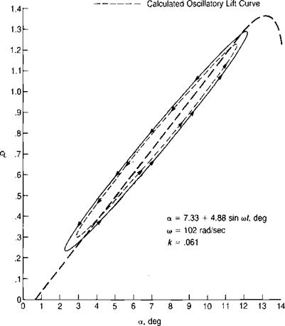
Static Lift Curve Measured Oscillatory Lift Curve
FIGURE 3.60 Correlation of Theory and Test Results for an Oscillating Airfoil |
Source: Liiva, Davenport, Gray, & Walton, “Two-Dimensional Tests of Airfoils Oscillating Near Stall,” USAAVLABS TR 68-13, 1968.
A A, = -60 (2 + |i2) CJo deg
Once the cyclic pitch that satisfied the moment coefficient criteria was established, the program evaluated the thrust, torque, and H-force coefficients.
The ability of the isolated rotor to overcome parasite drag if it were actually installed on a helicopter is given by the equilibrium equation:
fy Totj-j-p H
This can be nondimensionalized into a primary parameter, which appears on the rotor charts:
|
/M + (Ct/c)24 = 1* |
It is sometimes useful to have an indication of how close the rotor is operating to its capability. One such indicator is the angle of attack of the retreating tip:
<4270 = 0o + O i + B, + tan 1 —
і H
Another indicator that has been used is the maximum value of profile torque coefficient calculated at any azimuth position on the rotor:
 |
ACQ/o0= f ^-q° dr/R Jo dr/R
where
dCg/a0___ Ub p £
dr/R “TT f°
This parameter is computed at each azimuth during the integration for torque, and the computer can be made to remember the highest value obtained and to print it and its azimuth as part of the output.
For an analysis of a complete helicopter, the physical parameters of the main and tail rotors and the lift and drag characteristics of the airframe are used as inputs along with the gross weight, the forward speed, the atmospheric density, and the speed of sound. The program is made to iterate on 0O, А/, and 0Ot, as well as on Ax and Bx, to find the final trim conditions in a process identical to that used with the closed-form equations.
![]()
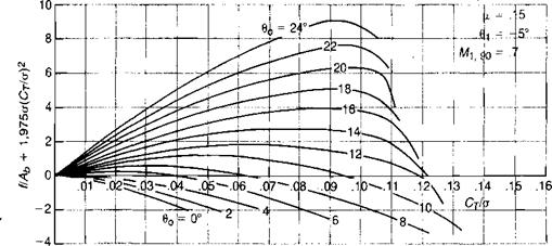
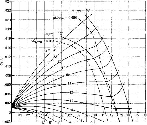
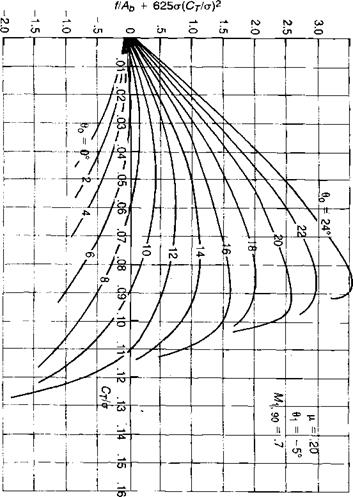
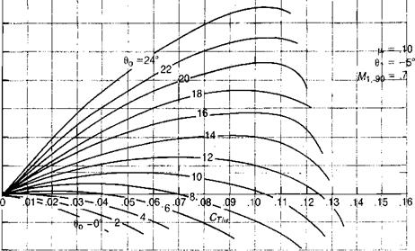
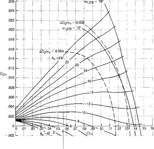
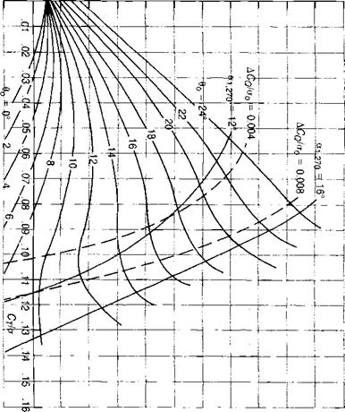
The charts at the end of this chapter have been produced with the methods just described and may be used to solve all of the common forward flight performance problems involving either main or tail rotors. The charts are based on a series of arbitrarily selected rotor parameters, although—as will be discussed—they are flexible enough to be used for rotors with different parameters.
The first chart of each pair can be used to obtain the power required in forward flight at a given tip speed ratio for known values of f/Ab, o, and CT/o. With these values defined, the top chart gives the collective pitch and the bottom chart the corresponding value of Cq/o. Two types of stall limits are shown on this chart: the angle of attack of the retreating tip, ali270, and the maximum value of the profile torque at any azimuth station, ACq/gq. Reference 3.46 uses values of 0.004 and 0.008 for ACq/gq as "lower and upper stall limits,” respectively, to indicate the region where many rotors begin to get into trouble because of stall effects. Most rotors can operate up to the higher set of limits as a helicopter rotor and well beyond it in the autogiro mode. The second set of charts can be used to obtain trim values of Q/o, А/, Ax — bXs, and Bx + aXj.
The charts have been constructed using the following rotor parameters:
Twist: —5°, linear
Airfoil: NACA 0012
Advancing tip Mach no: .7 (i. e., below the speed for compressibility losses)
Blade chord/radius ratio: 0.079
Tip loss factor: .97
None of these assumed parameters imposes significant limits on the use of the charts for rotors with different parameters. For rotors with twist other than
—5°, the charts may be used by referencing the collective pitch to the pitch at the 75% radius. The collective pitch to use with the charts is:
Ч_,.-0. + -7М0. + 5’)
For operation away from retreating blade stall, this is the only correction advised. For operation in the stall regime, twist affects the location of the limit lines of ACq/c0 and a1>270 on the torque plot. These limits move to higher values of CT/o for more than —5° of twist and to lower values for less twist. The displacement of the limit lines for other than —5° is approximately:
ACT/o = -0.003(0! + 5°)
The same displacement applies to the points on the torque curves where sudden changes in curvature occur because of retreating tip stall.
Many modern rotors have airfoils with higher stalling angles than the NACA 0012 on which the charts were based. These airfoils will also shift the limit lines and the points of sudden curvature change to the right. The magnitude of the shift can be estimated by the increase in the airfoil stall angle and by the distance between the two limit lines for (X1270 = 12° and (X1270= 16°.
Operation of the rotor at advancing tip Mach numbers that cause drag divergence can be accounted for using the method of Figure 3.43. This allows a correction to be made to the torque coefficient based on the amount the three- dimensional drag rise Mach number of the tip airfoil is exceeded. Thus the method can be used with airfoils other than the NACA 0012 if the airfoil drag characteristics are known.
The chord/radius ratio, c/R, enters into the analysis of unsteady aerodynamic effects both above and below stall. For the charts, a ratio of 0.079 was used. It will be assumed that these effects are small enough that the charts can safely be used for blades with other aspect ratios. Similarly, the tip loss factor of 0.97—which is a guess at any rate—can be assumed to apply to any reasonable rotor.
To illustrate the various uses of the charts, a series of numerical examples is given in Table 3.5.
The analysis so far has been based on the assumption that the lift coefficient on the blade element is only a function of the Mach number and of the instantaneous angle of attack corresponding to the component of velocity perpendicular to the leading edge. Correlation of the results of wind tunnel tests with the results of analytical studies based on this assumption give satisfactory agreement at low thrust levels, but at high thrust levels the analysis predicts lower thrust than is measured. One such comparison, taken from reference 3.33, is shown in Figure
![]()
|
|
|
3.54. The discrepancy is explained in reference 3.34 as primarily due to two effects: the beneficial effect of yawed flow on the maximum lift coefficient, and the finite time required for the boundary layer to separate during the stall.
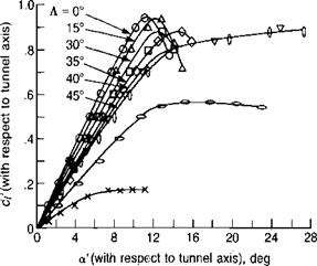
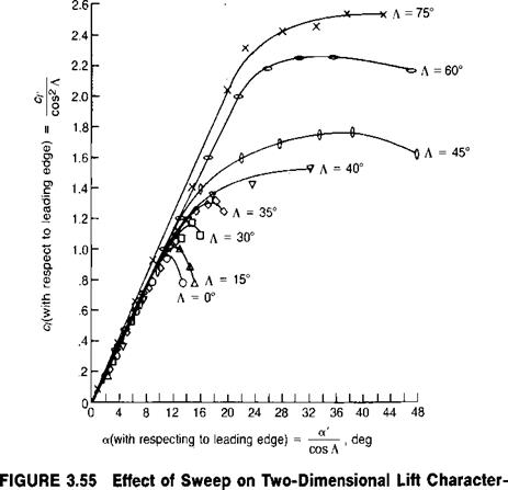
The significance of the yawed flow on maximum lift coefficient was first discussed in reference 3.35. The effect has been measured in wind tunnel tests of yawed wings. Figure 3.55 shows data from reference 3-36—corrected to infinite aspect ratio conditions—first as based on velocities and angles of attack referenced to the tunnel axis system, and then as based on the velocities and angles of attack perpendicular to the leading edge of the wing. In this latter system, which is consistent with that used in the blade element computing method, it may be seen that the measured maximum lift coefficient increases from 0.9 to 2.2 as the sweep is increased. Reference 3.35 suggests that the increase in maximum lift coefficient be represented by the engineering approximation:
|
FIGURE 3.54 Failure off Simple Theory to Correlate with Measured Rotor Thrust |
Source: Arcidiacono, “Aerodynamic Characteristics of a Model Helicopter Rotor Operating under Nominally Stalled Conditions in Forward Flight,” JAHS 9-3, 1964.
|
|
|
|
istics
Source: Purser & Spearman, “Wind-Tunnel Tests at Low Speed of Swept and Yawed Wings Having Various Plan Forms," NACA TN 2445, 1951.
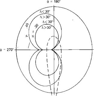
It is evident that there is no effect for the blade at |/ = 270°, where there is no yawed flow; but for other azimuth positions, the delay in stall can be significant. Figure 3.56 shows the regions on the rotor in which A exceeds 30° for tip speed ratios of 0.3 and 0.45. The effect can be considered to be important inside these boundaries. The increase in maximum lift coefficient can be incorporated into the airfoil data in a computer program in several ways.
If airfoil equations such as those in Chapter 6 are being used in the computer program, the value of aL, the angle of attack at which the airfoil first exhibits stall effects, an be modified by:
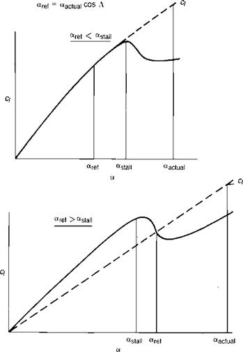
If tabulated airfoil data are being used, the effect can be incorporated by using a reference angle of attack that is less than the actual angle of attack:
a«f. = ttaamd COS A
|
ф = 0° V FIGURE 3.56 Boundaries for 30° of Local Sweep |
NUMERICAL INTEGRATION METHODS 219 This is used to define a fictitious lift curve slope such that:
|
|
If aref is less than the stall angle, the ct will be as if stall did not exist. If arcf is above the static stall angle, the ct will be somewhere above the static ch as shown in Figure 3.57.
The wind tunnel tests of reference 3.36 have also been used to determine the effect of sweep on the drag and pitching moment characteristics. These studies show that in contrast to lift, sweep angles under 60° have little effect on the drag and moment characteristics.
|
FIGURE 3.57 Use of the Reference Angle Concept |
If the angle of attack on a blade element is increasing rapidly, the stall will be delayed until some angle is reached considerably above the normal stall angle. An extensive discussion of this lift overshoot phenomenon is given in Chapter 6. Several ways of handling this effect have been developed for use in computer programs. These vary from the sophisticated analytical approaches of references 3.37 and 3.38 to the simpler empirical approaches of references 3.39, 3.40, and 3.41. The first two use potential flow and boundary layer equations to predict the separation angle and are not suited for programs whose primary objective is to calculate rotor performance. The last three depend on characteristics derived from oscillating airfoil wind tunnel tests, and each has been used in rotor performance programs.
The method of reference 3.39 calculates changes in the effective camber and angle of attack due to the pitching velocity and uses these with an empirical time lag to establish the characteristics of the lift overshoot and subsequent hysteresis loop boundaries.
The method of reference 3.40 makes use of tabulated lift and moment coefficients as a function of the angle of attack and its first two time derivatives. These supplement the usual tables, which are a function of angle of attack and the Mach number.
The final method was originally outlined in reference 3.34 and was later expanded in reference 3.41. It has been used to produce the isolated rotor charts in this chapter. In this method, the dynamic overshoot is expressed as an increase in stall angle due to a pitching velocity:
where у is a function of Mach number. It can be evaluated from wind tunnel tests of oscillating airfoils such as those reported in references 3.42 and 3.43 from those test points in which maximum lift was attained before the maximum angle of attack was reached. Chapter 6 has a discussion of this type of test. For the charts, a simple form of у given in reference 3.44 was used:
(.б
у = 1.76 In —
M
The term within the radical can be written as a function of the change in angle of attack from one azimuth position to another at the same radius station, since:
This angle – increment should be added to the static stall angle in whatever type of airfoil data presentation is used. If the equation form developed in Chapter 6 is used, Aasnll is simply added to aL after it has been modified for sweep effects. If tabulated airfoil data are being used, the stall delay can be incorporated using the technique that was used for the sweep effect—that is, by defining a reference angle of attack, which is now:
Along the boundary of the reverse-flow region, the calculated angle of attack, the sweep, and the rate of change of angle of attack on the blade element, are very high. This combination can result in the equations predicting unreasonably high—or low—lift coefficients. Even though the dynamic pressure is low along the boundary, significant errors can be introduced when an entire blade element is assigned a lift coefficient of 100 or more! For this reason, it has been found desirable to set bounds on the allowable lift coefficient. Figure 3.58 shows the limits on the minimum and maximum values that have been used for the 0012 airfoil. The maximum boundary is purely arbitrary and is based on a lift curve slope of 2tt and on the assumption that the sweep and stall delay effects will produce no benefits beyond an angle of attack of 45°. The minimum boundary represents the approximate lift characteristics of a sharp-edged flat plate with extreme thin airfoil stall characteristics.
In Chapter 6 it will be shown that the drag coefficient is affected by dynamic overshoot, which delays the drag rise in the same manner that it delays lift stall. The drag, however, is not affected by sweep as maximum lift is.
Another unsteady aerodynamic effect which may be included in the program is the classical unsteady potential flow. The lift of an airfoil is affected by the rate of change of angle of attack and by the rate of plunge, both of which produce shed vorticity lying behind the trailing edge, which induces velocities at the front of the airfoil. The basic theory was developed in reference 3.45. In that reference, potential theory was used to analyze the
In order to eliminate the imaginary terms, Да and 0 will be assumed to be pure oscillations at the rotor frequency, such that:
For use in the computing program, it is convenient to write the equation in terms of a correction due to unsteady effects, which can be simply added to the lift coefficient based on steady conditions. Assume that:
2V 2ClR Щ+Щ /иі+ Ul
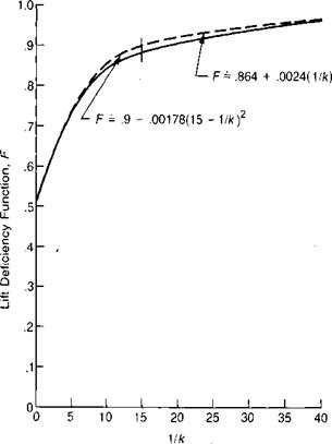
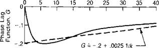
The functions F and G shown on Figure 3.59 can be approximated by:
If l/k < 15, then F = .9 – .00178 (15 – 1 Ik)2 If l/k > 15, then F = .864 + .0024 (l/k) and G = -.2 + .0025 (l/k)
These equations can be incorporated directly in the computer program. Figure 3.60 shows the correlation of the theory against the test results of an oscillating airfoil, which were reported in reference 3-42. It may be seen that the measured effect is somewhat greater than predicted. The relative importance of the effect on rotor performance is shown in Figure 3.61, where the calculated lift coefficient at the 75% radius for a typical flight condition is shown with and without the unsteady effect. The overall result is to increase the rotor thrust slightly for a given set of rotor conditions. The drag of the blade is assumed to be unaffected by the shed vorticity and, if required, the effect on aerodynamic pitching moment may be calculated using the methods given in reference 3-41.
For this analysis, the procedure used in deriving the closed-form equations will be modified somewhat by resolving both the lift and drag forces into a normal—or thrust—force where before only lift was assumed to contribute to thrust. Figure 3.52 shows the forces on a blade element.
The normal force coefficient is:
The contribution of the entire blade is:

|
r *о0. + л„) „ „Ьв+Уіо) і————————– I[4] – щ——————— |
 |
|
The integration can be performed by any of several methods suitable for numerical analysis. One of the simplest is Simpson’s rule. If the blade is evenly divided into ten elements from the center of rotation to the tip, the integration uses the eleven points calculated at the margin of each element:
The total thrust coefficient is the average of CT/o evaluated at N equally spaced azimuth positions around the rotor:
1 N
CT/o = —^ ACT/o,
N tl=l
The number of azimuth stations required is a matter of compromise between accuracy and computer time which will have to be made to satisfy the particular needs of the analyzer. (Our experience indicates that for most rotor conditions in which retreating blade stall is not a factor, eight azimuth stations are sufficient for engineering accuracy.)
![]()
The equivalence of flapping and feathering allows performance calculations to be based on a rigid rotor whose tip path plane is perpendicular to the shaft and whose pitching and rolling moments are trimmed out with cyclic pitch. These calculations will then apply to any condition in which the thrust and the angle of attack of the tip path plane are the same. The normal force coefficients are used to produce the pitching and rolling moment coefficient loadings:
![]()
and
The integrations for the entire moments are carried out with the same method used for thrust.
The chordwise force that contributes to torque and H-force is made up of three components: those due to pressure drag, skin friction, and tilt of the lift vector. In the closed-form derivation, pressure drag and skin friction were treated as one, being assumed to be governed by the component of velocity perpendicular to the leading edge. This is strictly otily true for pressure drag. Skin friction is a function of the magnitude and direction of the total local velocity as shown in Figure 3.52. The skin friction force, S. F., is:
S. F. = % cAr(U2T+ U2R)cf
where
UR = fJL cos ф
|
‘S-F – s/U+ Ul 2 The chordwise coefficient is: |
|
= – cArUr?U2r+ U c, |
The chordwise component of S. F. is:
![]() UT^U2T+ u
UT^U2T+ u
![]() -cArU2B
-cArU2B
2
 |
The total chordwise coefficient due to both pressure drag and skin friction
0 = 0O + ^ 0j – Ax cos |/ – Bx sin |/
0Т = Г£ + l sin \i
— V f
Up = ^ ~ Tlr У cos ^ ” ^a°cos ^
Where the closed-form equations can be used with sufficient accuracy for a0 and for vJClR:
2 CT/a 2sR а°~ЬУ a ~ (ClR)2
vJClR — C-r/o _
(The value of CT/a is initially either known or can be estimated from the closed – form equations. The value will be updated after the first full cycle of calculations.)
For cases in which the rotor has prescribed pitching or rolling velocities, the equation for Up is modified by adding:
r 0 г Ф.
Af/’ = Yficosv + lTnsmy
In these cases, trim is the condition in which the rotor aerodynamic pitching and rolling moments are equal to the rotor gyroscopic moments instead of to zero as in steady flight conditions. The gyroscopic pitching moment reacted on the shaft of a round flat disc that has a rolling velocity, Ф, is:
іМя„=уФП
where J is the polar moment of inertia. For a single blade instead of a disc, the equation becomes:
iVf^ = 2/,Ф П
 |
|
and
The blade flapping moment of inertia can be related to the Lock number:
![]() cpaR4
cpaR4
Y
 |
||
Similarly
The rotor is in trim when:
^Лі/^ісго + См/Ggyro — 0 <
Ск/®ісго + ^fl/^gyro = 0
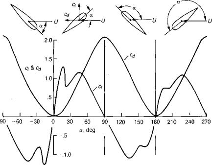
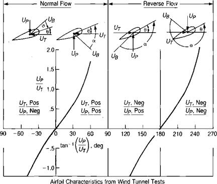
Since the sign and magnitude of a can vary widely over the rotor disc, it is necessary that the airfoil characteristics be defined throughout the entire range. Figure 3.53 shows the relationships between the angle of attack and the ratio of UP to UT. Also shown are the lift and drag coefficients of an NACA 0012 airfoil measured in a wind tunnel and reported in reference 3.32. When the airfoil characteristics are used as a function of a with the signs as shown, the normal and chordwise force equations will automatically resolve the lift and drag components into forces with the correct orientation. (Note: for the cases where UP and UT are both negative, the angle is in the third quadrant and computers will usually assign it a minus sign—for example, —135°. It is necessary in this procedure to add 360° so that the third quadrant angle is positive—for example, 225°.) The airfoil lift and drag coefficients can be written as equations that are a function of a, and the local Mach number, M, by the method outlined in Chapter 6. The local Mach number is:
![]() UBClR
UBClR
Speed of sound