Category Helicopter Performance, Stability, and Control

The trim conditions in level flight have been calculated while eliminating the assumptions one at a time. The results are shown in Table 3.4 for tip speed ratios of 0.30 and 0.45. (In reality, the trim conditions at the tip speed ratio of 0.45 are unobtainable for the example helicopter because of excessive blade stall, as will later be shown; but as a basis of comparing the effects of the various assumptions, it is an illustrative case.) It may be seen from Table 3.4 that the elimination of the assumption that there are no root or tip losses makes relatively little difference in the trim conditions at the low speed but makes a significant difference at high speeds. This is due to the large reduction in the H-force and the consequent reduction in the nose-down attitude of the rotor. The reduction in H-force can be traced to the variation in the calculated induced drag in the tip annulus as a function of azimuth position. Because of the higher dynamic pressure on the advancing tip, the induced drag is higher on the advancing side, where it contributes to positive H-force, than it is on the retreating side, where it contributes to negative H-force. Thus the elimination of the induced drag in this annulus by considering it lost due to tip effects results in a net decrease of the calculated H-force.

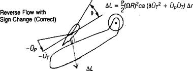
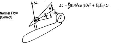
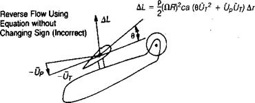
The effect of treating the reverse flow region correctly is shown in Table 3.4. At a tip speed ratio of 0.3, the main rotor power is increased approximately 6%, but at a tip speed ratio of 0.45 it is decreased about 10% compared to the corresponding calculation with the reverse-flow region treated incorrectly. At the lower speed, the increase in rotor thrust in the normal-flow region requires higher power. At the higher speed, the reduction in the H-force due to the reversal of the lift vectors in the reverse-flow region, as shown in Figure 3.50, has resulted in a large reduction in the rotor angle and thus has put both the rotor and the fuselage into a more favorable condition with respect to overall power.

The use of a three-term drag polar in place of an average value has an effect similar to those caused by eliminating the first two assumptions—relatively little effect at the low speed, but a dramatic decrease in rotor power at the high speed. Again, this reduction can be traced to the decrease in H-force and the more favorable rotor and fuselage attitude that results. Paradoxically, this is due to the increase in drag on the retreating side, where the contribution to H-force is negative.

The logical next step would be to present all the closed-form rotor equations with the assumptions eliminated. This step, however, has been bypassed in favor of developing the charts at the end of this chapter, which are based on a digital computer program. This program, in using rigorous equations for the

forces at the blade elements, automatically eliminates the assumptions while also including the effects of compressibility and unsteady aerodynamics, which are difficult to include in any closed-form analysis.

Numerical integration methods use the same basic equations for the forces on a blade element as do closed integration methods, but because of the nature of the computer, which doesn’t mind boring, repetitive computations, fewer assumptions need be used. A primary advantage of these methods is their ability to use two – dimensional airfoil data as a function of angle of attack and Mach number throughout the complete ranges of these two parameters as they exist on the rotor. In addition, the methods can be made—with ever-increasing complexity—to handle unsteady aerodynamics, yawed flow characteristics, complicated induced velocity patterns, blade flexibility, and lifting surface (rather than lifting line) aerodynamics.

A requirement of any program is that it have the capability to find the trim condition in which the blade inertial, centrifugal, and aerodynamic forces and moments are all in equilibrium, as they must be for a rotor in steady flight. There are two starting approaches for a hinged rotor. In the most common, the computer calculates the flapping by following one blade around the azimuth while continually evaluating its flapping acceleration, velocity, and displacement. For a reasonable set of shaft angles and control settings, the calculations will converge on a condition where the flapping repeats itself from one revolution to another. The other blades in the rotor are assumed to fly in the same path. This method is sometimes referred to as a flapdoodle. If it is required to trim the first harmonic flapping to zero with respect to the shaft, the computer changes cyclic pitch in a logical way to do this. Once this condition is achieved, the flapping hinges could be locked. In this situation, the longitudinal and lateral hub moments would be zero, since the tip path plane is perpendicular to the shaft.

The second method—and the one that will be used here—obtains the same results by starting first with locked hinges. On this rotor, changes in cyclic pitch result in aerodynamic pitching and rolling moments. The computer searches for the cyclic pitch that reduces these moments to zero, thus giving the same results as those obtained with the more common method. Because of the equivalence of flapping and feathering demonstrated in the previous analyses, the trim values of cyclic pitch can be reidentified as (Вг + ax ) and {Ax — bj) and thus applicable to flapping rotors in which the tip path plane is not necessarily perpendicular to the shaft.

The second method gives the same results as the first except for the loss of flapping harmonics above the first. Studies have shown that these have little effect on rotor performance, so their loss is not serious for our purposes. Comparison of the two methods indicates that the second is more economical in computer time and will often converge to a trim solution at extreme conditions, where the flapdoodle procedure will diverge because of second-order effects.

The method outlined in the following paragraphs is suitable for a medium­sized computer and is based on the following limitations and assumptions:

• Obtaining performance and trim conditions is the primary objective.

• Two-dimensional airfoil lift and drag characteristics are available.

• The blades do not bend or twist elastically.

• The induced velocity distribution is given by the equation:

( r.

VL = v I 1 + ——————— Sin |/ I

Another refinement to the closed-form equations involves the use of an expression for the coefficient of drag as a function of the local angle of attack rather than of a single average value. The classical form, which was discussed in Chapter 1, is the three-term power series—usually referred to as a three-term drag polar:

o = o0 + (dfi + cda2 where a is in radians and the constants are picked to make the best fit with two – dimensional airfoil data. The profile torque and H-force coefficient equations without reverse-flow considerations but with the three-term drag polar are:

2 36 4

*VC« ~ ) ~~ Iі + Ю + —l— к l+-u2L

e:|i

55 2> i >>J i + V

2 V

+ 0,А'(—2 + Зр2)

1 + – р

2

Airfoil data are usually better fit with a power series with more than three terms, but the use of any power above the second leads to difficulties in the integration which do not justify the increased accuracy that might result. The three constants

in the drag polar should be chosen to fit the airfoil data at a representative Mach number corresponding to 75% of the tip speed and the highest angle of attack on the retreating side. A discussion of the problem of fitting a three-term polar to test data was given in Chapter 1, and Figure 1.37 shows three polars that approximate the NACA 0012 data.

In Chapter 1, a tip loss factor to account for the gradual falling off of the lift at the tip was used in the integration for hover thrust, and an approximate method was given for evaluating the tip loss factor as a function of the thrust coefficient and the number of blades. The same phenomenon exists in forward flight, but there is not yet any comparable method of evaluating the tip loss factor. Nevertheless, the need is recognized, so the closed-form equations are often derived using BR as the

upper limit of integration, and calculations are based on the value of В obtained with the hover equation or with an arbitrary constant such as 0.97. When the tip loss factor and

or

These equations are more complicated looking than the corresponding equations without tip and root losses; but since В and x0 are constants, the resulting numerical equations, which are actually used for calculations, are no more complicated.

Reverse-Flow Region

The integration process used so far has ignored the reverse-flow region, shown in Figure 3.14, by integrating around the azimuth from zero to 2n with no regard for the fact that in the reverse-flow region this method assigns the wrong sign to lift forces, as shown in Figure 3.50, and thus results in a calculated thrust value that is too high. For small tip speed ratios (less than about.25), the error is insignificant since both the size and the dynamic pressures in the reverse-flow region are small. At higher tip speed ratios, however, the error becomes more and more significant. The deficiency can be corrected during the integration by dividing the rotor into three regions, as shown in Figure 3.51, each with its separate limits of integration. Using this method, the thrust equation becomes:

FIGURE 3.50 Illustration of the Sign Change Required in the Reverse Flow Region

The resulting equation for CT/o is:

a 4л

CT/a

The basic mechanism of autorotation in vertical flight was described in Chapter 2. Autorotation in forward flight is based on the same concept—that over the entire rotor, the integrated effect of the tilt of the lift vector at each blade element is sufficient to overcome the integrated effect of the drag at all of the blade elements.

The closed-form equations can be used to calculate the autorotative rate of descent and the trim conditions in forward flight. Two calculating methods are available; the first consists of using the previous method for climb and descents by assuming several rates of descent and plotting main rotor power versus rate of descent. The rate of descent for which the main rotor power is zero—or a small negative value required to overcome losses—is the autorotative rate of descent.

The fuselage lift and drag are a function of the angle of attack of the fuselage where—assuming that the rotor downwash at the fuselage is equal to the momentum value at the rotor:

The calculation has been made for the example helicopter assuming that transmission and accessory losses amounted to 15 h. p. The results of the calculations are listed in Table 3.3.

The rate of descent in autorotation could have been roughly estimated from the power required in level flight and the rate of change of potential energy required to produce this power:

33,000 h. p.
G. W.

The calculated power required for level flight (including 15 h. p. for transmission and accessory losses) is 1,137 h. p. The corresponding estimated rate of descent is

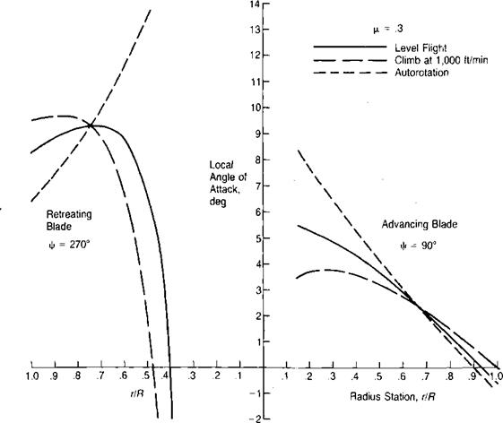
1,880 ft/min. Comparing this with the calculated rate of descent of 1,790 ft/min indicates an "efficiency” of 105%. The apparent gain is primarily due to the reduction in the negative lift on the fuselage and a reduction in the tail rotor Id – force. This value can be used for rough estimates of the autorotative rates of descent of the example helicopter at other weights and forward speeds in the neighborhood of 115 knots. The angle of attack distribution in Figure 3.48 shows that the angle of attack is decreased on the retreating tip but increased inboard compared to level flight. For this reason, some helicopter aerodynamicists consider that the critical position on the retreating blade in autorotation is the station at which the tangential velocity is 40% of the tip speed, or:

r/Ra«. = 0.4 + Ц

if the local angle of attack exceeds the stall angle of the airfoil at this station, high drag can be expected to compromise the ability of the rotor to sustain autorotation.

Up to this point, the closed-form equations have been kept simple in order to illustrate the derivation and to produce results that can be readily used for quick calculations. The primary assumptions that have been used are:

• There is no tip loss or root cutout.

• The reverse flow region is ignored.

• A constant blade element drag coefficient is used.

When one or all of these assumptions are eliminated, the accuracy of the method is improved but the work in deriving the equations becomes greater, and the equations themselves become more unwieldly to use. In order to evaluate the effects of the assumptions, they will be examined one at a time.

The closed-form equations can also be used to calculate the power and trim conditions in a climb or in a descent by incorporating the component of gross

weight that acts along the flight path in the equation for the angle of attack of the tip path plane. Figure 3.49 shows the force balance in a descent and in a climb. The equation for the equilibrium tip path plane angle of attack—using the same derivation as in forward flight—is:

PF + HM + HT + G. W. sin у
G. W. — LF

where

with the rate of climb, R/C, in feet/minute and the forward speed, V, in feet/second. The trim conditions for the example helicopter at 115 knots (|l = .3)

and at a rate of climb of 1,000 feet/minute have been calculated by the same iterative method used for level flight. The results are shown in Table 3.3 and the angle of attack distribution in Figure 3.48.

The difference in power required to climb compared to that required for level flight could have also been roughly estimated from the rate of change of potential energy:

R/C( GW)

33,000

For this case, the estimated difference in power is 606 h. p., whereas the calculated difference (including the tail rotor) is 668 h. p. Thus the example helicopter has a

climb efficiency of 91%. Most of the loss of efficiency can be attributed to the increased fuselage negative lift while a smaller part is associated with the increased tail rotor H-force. This value of efficiency can be used to make rough estimates of the increment in power required to climb at other weights, rates of climb, and speeds in the neighborhood of 115 knots.

Level Flight

Since the trim conditions are dependent on each other, the calculations are done as an iteration of the angle of attack of the tip path plane and the rotor thrust, using the equations:

Df + Нм + Ht G. W. – Lf

T = ^(GM. – LPy + (Df + HM + HTy

The fuselage lift and drag characteristics as a function of angle of attack of the fuselage may be estimated from previous experience or measured in a wind tunnel. Typical fuselage aerodynamics that will be assumed to apply to the example helicopter are shown in Figures A2 through A4 of Appendix A. The lift and drag forces are:

Lp = q(Lp/q)

Df = qf

where the fuselage angle of attack is:

Ctf = CtTPp — is ais ~ A&d. w.

where AaD W is the downwash angle produced at the fuselage by the rotor. A wind tunnel investigation reported in reference 3.31 shows that the rotor downwash at the fuselage is approximately equal to the value corresponding to the momentum – induced velocity at the plane of the rotor:

Thus

aF = — — іs — a! radians Iі

Trim conditions for a helicopter can now be evaluated from the equations just developed. A typical case for the example helicopter has been prepared. The assumptions that were used in the iterative process were:

First Iteration Subsequent Iterations

« = H = (H0 + H()prcv iter

= ® Clp — (Qp)prcv. iter.

The results of the calculations are shown in Table 3.2.

Figure 3.48 shows the distribution of the local angle of attack along the advancing and retreating blades for level flight and the two other flight conditions to be discussed next. For the example helicopter with 10° of twist, the highest local angle of attack is not at the retreating tip but at the 70% station.

The tail rotor is a flapping rotor without cyclic pitch and is thus similar to the early autogiro rotors for which the blade element theory was originally developed. (Note: Even in tail rotors that have no hinges and are thus classified as rigid rotors, the aerodynamic and centrifugal forces generally predominate over the structural stiffness, and the rotor will flap by bending the blades almost as much as if it had actual mechanical hinges. The equations developed here can, therefore, be assumed to apply in the first approximation to these rotors.) Most tail rotors—and some main rotors—are designed with a mechanical coupling between flapping and feathering such that a change in flapping produces a change in feathering:

A0 = AP tan 53

where 83 is the slant angle of the flapping hinge as shown in Figure 3-45. The angle shown there is negative, which is the usual (but not the universal) application on tail rotors. The local blade pitch angle is:

T

0 = (0O + a0 tan 53) +0!—————- ax tan 53 cos |/ — bx tan 83 sin jf

R

The last two terms have the form of cyclic pitch and can be used in the basic rotor equations by treating them as such:

A, = a. tan53

leff. J

Van8>

Unlike the case of the main rotor, where the angle of attack of the tip path plane is known from equilibrium conditions, for a tail rotor the angle of attack of the shaft is known. It is generally zero unless the tail rotor shaft is deliberately tilted or the helicopter is flying with sideslip. For this reason, the tail rotor equations are written in terms of the inflow ratio, X.

where the subscript T denotes that all parameters refer to the tad rotor. Table 3.1 shows the trim conditions for the tail rotor of the example helicopter at 115 knots for 83 values of 0°, 30°, and —30°. It may be seen that the effect of the delta-three

hinge on the trim conditions is small enough to be considered negligible for performance calculations.

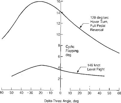
Although it has little effect on steady-state conditions, the delta-three angle is important in reducing flapping during maneuvers. Figure 3.47 from reference 3.30 shows that both positive and negative values are effective.

Source: Huber & Frommlett, “Development of a Bearingless Helicopter Tail Rotor,” 6th European Rotorcraft Forum, 1980.

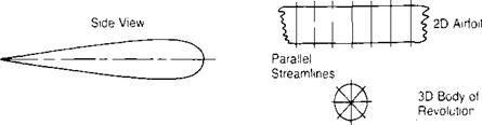
If any blade eement exceeds the drag divergence Mach number for its airfoil, the power required will be higher than that calculated from the closed-form equations. Before developing the method for estimating this power loss, it is appropriate to discuss the three-dimensional phenomenon known as compressibility tip relief.

The relief effect is seen clearly by comparing the streamlines on a two – dimensional airfoil and on a three-dimensional body of revolution with the same thickness ratio shown in Figure 3.37. On the two-dimensional airfoil, the streamlines are constrained to remain parallel to each other but on the body of revolution, they spread out as they approach the maximum thickness thus reducing the local velocity and increasing the free-stream Mach number at which drag

divergence occurs. The blade tip may be thought of as a combination of a two* and three-dimensional body and, as such, would be expected to have a drag divergence Mach number that lies between those of the other two bodies. Wind tunnel tests of wings, reported in reference 3.20, verify this expectation by showing that the drag divergence Mach number increases as the aspect ratio is decreased.

Tip rebel consists of two parts: a large one due to the reduction of the effective Mach number, which delavs the formation of the shock wave, and a smaller one due to the reduction in the local dvnamic pressure, which reduces the actual drag and, thus, the drag coefficient based on the free-stream dynamic pressure.

A method for estimating the tip relief for rotor blades is given in reference 3.21 based on the similar analvsis for wings of reference 3.22. With this method, both the reduction of Mach number and that of drag coefficient may be calculated as a function of the blade thickness ratio and the distance from the tip. The method is suitable for detailed computer studies, but for a quick estimate of tip relief, a simpler method is available. The simpler method is based on the fact that the tip of a blade with a thick airfoil will act more like a three-dimensional body and thus will have a greater tip relief than the tip of a blade with a thin airfoil. A convenient velocitv parameter that is a function of the airfoil thickness ratio is the incompressible two-dimensional velocity ratio, (z F), and the average of this ratio along the chord is used to define the effective Mach number at the tip.

M

The local velocity ratio, г/V, as a function of chord can be calculated using airfoil theory or can be derived from wind tunnel measurements of the pressure

coefficient distribution since:

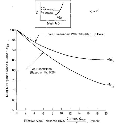
For many airfoils, the local value of {v/Vj1 is plotted against chord in Appendix I of reference 3.23. These plots have been used to find the average velocity ratio at zero angle of attack and the corresponding tip relief for several families of airfoils. The correction has been applied to the test data shown in Figure 6.28 of Chapter 6 to produce Figure 3.38, which shows the two – and three – dimensional drag divergence Mach numbers as a function of the effective thickness ratio. The method has been used to correlate with flight test data given in references 3.24 and 3.25. The results shown in the following table demonstrate a satisfying degree of agreement.

A further check has been made applying the method to the fixed-wing example of reference 3.22. For this case, the wing had a NACA 0012 airfoil and an aspect ratio of 3.25. The method of this section was adapted to the wing by assuming that the tip relief linearly decreased to zero one chord length in from each tip. The average Mach number relief for the wing, therefore, was less than the extreme tip value. Figure 3.39 shows the experimental drag measurements for the

Airfoil — NACA 0012

Source of test data: Anderson, "Aspect Ratio Influence at High Subsonic Speeds,” Jour, of Aero. Sci. 23-9, 1956.

low-aspect-ratio wing and estimates for a wing of infinite aspect ratio using both the sophisticated method of reference 3.22 and the simple method of this section. Again, the degree of correlation is satisfactory at least near the drag rise area, which determines the drag divergence Mach number.

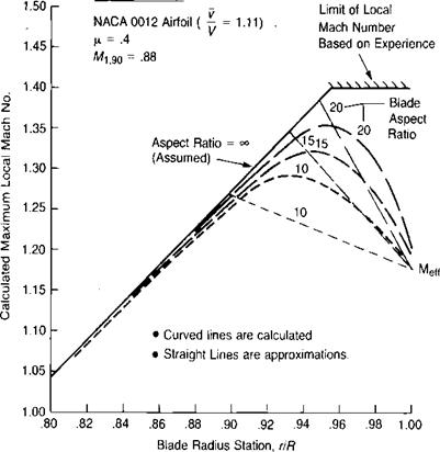
Additional justification of the procedure is developed by comparison with calculations of the spanwise distribution of the maximum local Mach number for blades of aspect ratios of 10,15, and 20, shown in Figure 3.40 taken from reference 3.26. The airfoil is the NACA 0012. The calculated curves are compared with straight lines, which follow the assumptions just discussed. The assumptions appear to be very good for the aspect ratios of 15 and 20, though somewhat extreme for the – aspect ratio of 10.

An approximation to the additional torque due to compressibility may be obtained by integrating the extra drag from the radius station at which the drag first rises above the incompressible value to the tip. In forward flight, the advancing tip normally operates at very low angles of attack so that to a first approximation, the compressibility losses can be related to the airfoil drag characteristics at zero lift. Test results show, however, that the losses are also a function of CT/o. The procedure adopted for this analysis has been to derive the

basic equations using the zero-lift drag characteristics of the airfoil and then to establish an empirical correction to the drag rise Mach number as guided by wind tunnel and flight tests of actual rotors producing thrust.

The geometric relationships that enter into the analysis are shown in Figure 3.41, where (r/R)dr is the radius station at which drag rise is first experienced and ф, and i|/2 are the azimuth angles bounding the drag rise region. The equations for these two parameters

and Mdr is the Mach number at which drag rise first appears.

The drag increment, Acd, is a function of Mach number. Figure 3.42 shows the drag for a

The value of Mdr is a function of the spanwise position of the blade element, being the two-dimensional value, M*, inboard of one chord length, and being the three-dimensional value, ЛЦ, at the tip. Thus for the inboard section:

-< i–

R R

and for the tip section:

With these relationships, it is possible to evaluate the quantity, (ACQ/<Jcomp)/Mn/, as a function of the airfoil characteristics, Kx and MdrjMdrj the chord to radius ratio, c/R; and the flight conditions, MdrjMm, and jx. As an example, the integration has been carried out assuming the 0012 airfoil with:

(Assume Л1*/ЛЦ = ЛЦ/ЛЦ from Figure 3.38.)

Figure 3.43 shows the results of this integration in terms of the amount the advancing tip Mach number exceeds the three-dimensional drag rise Mach number. Although Figure 3.43 is based on the 0012 airfoil, it should be valid enough as a first approximation to be used with other airfoils suitable for rotors using either two-dimensional wind tunnel results or the value of Л1* from the upper portion of Figure 3.43, which has been generated using figures 3.38 and 3.42 as guides.

The effect of CT/o on compressibility losses has been incorporated into the method after examining the full-sale wind tunnel results of reference 3.27 and the flight test results of reference 3.28. Although there is not complete consistency between the various sets of test data, a reasonable approach appears to be to assume that Л1* has the form:

Ж*, = Md [1 – 6(CT/a)2]

3 3ci=0

Satisfactory correlation of the method with wind tunnel test results is shown in Figure 3.44.

For those more sophisticated rotor analyses using computers with stored tables of two-dimensional lift and drag coefficients as a function of angle of attack

and Mach number, the tip relief may be accounted for by calculating an effective Mach number for the blade elements within one chord length of the tip such that:

Source: McCloud, Biggers, & Stroub, "An Investigation of Full-Scale Helicopter Rotors at High Advance Ratios and Advancing Tip Mach Numbers," NASA TN D4632, 1968.

This effect can generally be easily incorporated in the program by definin an effective speed of sound for the outboard elements such that:

Speed of soundcff = Speed of sound2Ct

A further complication of the whole question of drag divergence on the advancing tip is the evidence that there is a finite delay in compressibility effects

due to the rate of change of Mach number with time. Wind tunnel tests of a nonlifting rotor reported in reference 3.29 indicate that the maximum com­pressibility effects occur somewhat later than |/ = 90°, where the local Mach number is the highest. There is not yet any simple method for accounting for this effect.

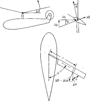
The H – force is the horizontal force perpendicular to the rotor shaft and is derived in the same manner as that of the torque. Figure 3-35 shows the arrangement of the forces on the blades that contribute to the H-forces. At any blade element the incremental H-force is:

AH = f AD – AL — ] sin у — ALB cos у

uT)

In level flight, AH is positive on the advancing side and negative on the retreating side, although in autorotation the reverse can be true. Thus the total H-force can be either positive or negative, depending on which side of the rotor is dominant.

Because of this, the magnitude of the calculated H-force can vary drastically with relatively small changes in flight conditions—or, as will be shown later, with changes in the assumptions made in the integration. When the integration is carried out with the same assumptions as for the thrust and torque equations, the result is:

9. + -7-) _ + a0

—a,

1U { ^0 З Ш 2

Again, using the equations for (Bl + al) and (Д — and also the equation for CT/o, the equation simplifies to:

i + JL + A^+I _!■_ 2 9 2 / 3 CLR 8 CLR

4 1 + |T

In this case the last term is generally small but perhaps not negligible. If the inflow portions of the rotor equations are combined, it may be seen that:

£q/Ginflow — ^ CT/0 + a Ct/g)

This identity is illustrated graphically by examining the rotor mounted in a wind tunnel at a positive angle of attack, as shown in Figure 3.36. The momentum power that the rotor extracts from the airflow is negative rotor power and is equal

The solution of the closed-form blade element method for the torque required in forward flight follows the procedures developed for torque in hover and for thrust in forward flight. The increment of torque as shown in Figure 3.35, is:’

AQ = r(AD – AL<|>) = Jad – ДL ^j

^ Л L FIGURE 3.35 Force Increments Acting on Blade Element Which Contribute to Rotor Torque and H-Force

Carrying through the integration and nondimensionalizing gives: Ct/a = — (1 + Ц2) – – І (Xі – |i«, )2 + – fia, (V – |i a.) 8 4 l 2

a Iі a 4 2 8

M/ 3 CLR (The equation has been written in this form to show the equivalence with the similar equation in reference 3.17).

The first part is the profile torque coefficient due only to the drag coefficient, and the second part is the inflow torque coefficient due only to the tilt of the lift vector. The inflow term includes both the induced and the parasite contributions as defined by the momentum equations. It can be simplified by using the equations for (Bl + ax) and (Д — bx) previously derived. With this substitution, all of the cyclic pitch and flapping terms drop out:

2 9 2 ) 3 CLR 8 CLRj

The last term, which is a function of a0 and Vy/CLR, is generally negligible when compared with the other terms. For this type of analysis, the value of cd to use is the average obtained as a function of CT/o as it was in hover—that is, as a function of angle of attack equal to 57.3 (Ct/g) degrees and at a Mach number corresponding to 75% of the tip speed. A more sophisticated way of handling the drag coefficient will be discussed later.