Our heavyweight helicopter equal in the world does not have
In Rostov started production of the most load-lifting rotary-wing car The Russian holding «Helicopt[...]

Everything about aircrafts and helicopters. News and events in aviation worldwide. Civil, transportation, military helicopters and airplanes.

Everything about aircrafts and helicopters. News and events in aviation worldwide. Civil, transportation, military helicopters and airplanes.

Everything about aircrafts and helicopters. News and events in aviation worldwide. Civil, transportation, military helicopters and airplanes.

Everything about aircrafts and helicopters. News and events in aviation worldwide. Civil, transportation, military helicopters and airplanes.


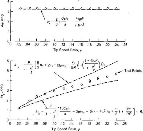 |
Reference 3.5 presents flapping obtained during a wind tunnel test of a model rotor at low tip speed ratios. The measured values of coning, longitudinal flapping, and lateral flapping are shown in Figure 3.34 along with values calculated from the
![]()
![]()
![]()
 + Ал
+ Ал
Tip Speed Ratio, |i
FIGURE 3.34 Measured and Calculated Flapping for Wind Tunnel Model
Sources: Harris, “Articulated Rotor Blade Flapping Motion at Low Advance Ratio,” JAHS 17-1, 1972; Johnson, “Comparison of Calculated and Measured Helicopter Rotor Lateral Flapping Angles,” AVRADCOM TR 80-A-11 NASA TM 81213, 1980.
equations derived here. Two calculated lines are shown for longitudinal flapping. The first is based on the equation derived earlier and the second on an alternative form generated by combining the equations for ax and CT/o:
![]()
![]() 6CT/o
6CT/o
1–ЄІ L
2
This second equation gives lower calculated flapping because the wind tunnel model produced a somewhat lower value of Cx/a than would be predicted from the test conditions. (This correlation of longitudinal flapping is slightly different from that given in reference 3.5 because of a term equivalent to 4|i2(90 + jdx) was omitted from that study.)
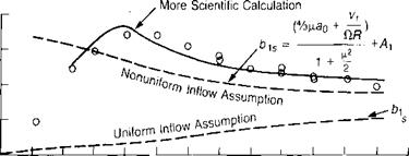
The presence of the term vJClR in the lateral flapping equation is the result of assuming that the induced velocity distribution is nonuniform—specifically, that it has the form:
V, =VA 1 + К———————- COS 1/ )
* /
where К is assumed to equal to unity. The assumption is obviously not valid near hover, as shown in Figure 3.34, but above a tip speed ratio of about 0.05 it gives better correlation than the calculations based on uniform inflow. More detailed analysis of the role of the induced velocity distribution will be found in references 3.5 and 3-6. The large lateral flapping at low forward speeds requires left cyclic stick to trim the helicopter (for rotors turning counterclockwise). (Pilots refer to this as the "transverse flow” effect.) The magnitude of this cross-coupling effect is shown by the lateral flapping equation to be a function of vu which in turn is a function of the disc loading. In sideward flight, forward stick must be held in flight to the right and aft stick in flight to the left. This effect is discussed in reference 3.18.
A much more scientific approach can be used—one involving a free wake analysis—as is reported in reference 3.19. This results in an almost perfect correlation with the wind tunnel data for lateral flapping.
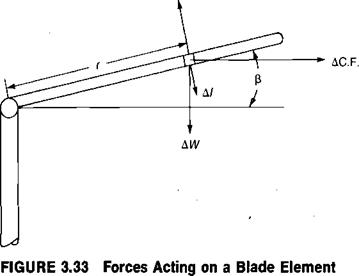
An expression for the steady portion of blade flapping, or coning, <?0, may be derived in forward flight using the same procedure as was used in hover—that is, setting all of the blade bending moments to zero at the hinge. Figure 3.33 shows a rotor blade with aerodynamic, weight, inertial, and centrifugal forces acting on a blade element. At the flapping hinge—which for this analysis will be assumed to be at the center of rotation—the net moment must be zero since a hinge cannot support a moment. The equations for the four moments are:
 , R2
, R2
mg rar — —mg —
![]()
|
|
|
|
|
|
|
|
|
|
|
|
|
|
![]()
Since only the steady portion of the flapping is being derived, only those terms that do not contain sin j/, cos j/, sin 2 j/, or cos 2 j/ need be retained. When MA is expanded and the trignometric identity
The constant portion of the weight equation is simply:
![]() mgR2
mgR2
Note that this is identical to the equation for coning derived for the hovering rotor with ideal twist. Although this equation has been derived for a rotor with flapping hinges, it is a good assumption even for two-bladed teetering rotors and for rigid rotors, since the aerodynamic and centrifugal forces overpower whatever structural stiffness the blades may have.
Generally in a helicopter analysis, the value of Ct/g is known from its definition:
and thus the primary use of the equation for CT/o is to determine the collective pitch, 0O, which will be used in subsequent analysis:
3 3 2
The longitudinal cyclic pitch Bx has already been derived:
The magnitude of the flapping, alp is determined by the pitching moment that the rotor must produce to balance such things as an offset center-of-gravity position, a
lift force on the horizontal stabilizer, and/or an aerodynamic pitching moment on the fuselage. If the net of these effects is zero, then ax will also be zero. If the net effect is not zero, ax can be evaluated by the methods derived in Chapter 8, "The Helicopter in Trim.”
 |
|
For some types of problems, such as determining the stability and control characteristics of the rotor or for calculating the flapping of a tail rotor or of a rotor in a wind tunnel with fixed cyclic pitch, it is convenient to rewrite the equation in terms of the angle of attack of the plane perpendicular to the shaft, a„ rather than the angle of attack of the tip path plane. In this case:
The equation for the lateral cyclic pitch, Ax> may be derived by setting the pitching moment on the rotor to zero. The result is:
where the lateral flapping, bx , is that required to trim the helicopter for external rolling moments such as those produced by tail rotor thrust or a lateral center of gravity offset. For most steady flight conditions, bls can be considered to be negligible.
![]()
In Chapter 1 it was shown that if each blade element operated at the same lift coefficient, ~ch a relationship with Ct/g could be established that helped give a feeling for how close the rotor was to stall:
A similar calculation can be made in forward flight, although it must be admitted that the usefulness is somewhat limited considering that in forward flight the stall is localized on the retreating side. Let
Т = —[П f * – U2T7t сігіщ
2" J, l 2
Cr/a = — Г" [‘ Vd — iy
then
![]() -4 l+-p’ 6 2
-4 l+-p’ 6 2
Just as in hover, the rotor thrust in forward flight can be computed from the integration of the lift on each blade element along the blade and around the azimuth. The same equation for the incremental lift applies:
A L = qctcAr
or in terms of blade element conditions:
AL = – UladcAr 2
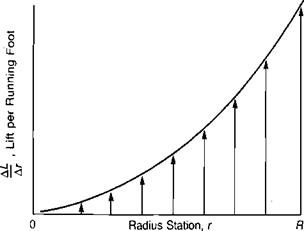
where both the velocity, UT, and the angle of attack, a, have been derived as functions of r/R and of j/. The integration procedure is simple in principle but tedious in application because of the large number of terms involved. For this reason, the method will be outlined in general, but detailed steps will be left to the ambitious student. The integration starts with the equation of lift per running foot:
AL p tt2
a — acUr Ct Ar 2
For a given value of j/, the lift per running foot is as shown in Figure 3.32. The lift on the blade is designated as Lh and is the area under the curve.
![]() * A L
* A L
|
|
|
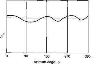
For each value of j/, the integral can be evaluated and the result plotted as a function of \l, as in Figure 3.32. The average lift per blade, Lb, around the azimuth is the area under the curve divided by the length of the horizontal axis which is 360° or 2n radians:
![]()
![]() L>/4
L>/4
Substituting for Ly the average lift per blade becomes a double integral on r and J/. The total thrust is equal to the number of blades times the average lift per blade:
In
this stage of the analysis and discussed later along with the effect of the reversed flow region.)
 |
|
The integration is straightforward and may be done using tables of integrals. The result is:
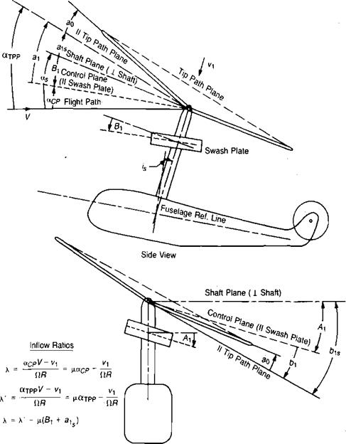
The term, СЦ-рр — (Bl + <*!), is the angle of attack of the swashplate or control plane with respect to the flight path, as shown in Figure 3.30. In classical treatments of rotor aerodynamics, such as in references 3.16 and 3.17, the flow perpendicular to this control plane is called the inflow:
Inflow = F[aTPP — (B, + )] — vy
and normalizing by dividing by tip speed gives the inflow ratio, X:
X=(l[aTPP – (B, + at)]~ vJClR
or in terms of shaft angle:
X=i[a,-BA-vJdR
As a function of 0, |i, and X, the thrust coefficient is:
This form is convenient when working with flapping rotors without cyclic pitch such as tail rotors or the rotors of simple autogiros. It is, however, somewhat awkward to use for the analysis of helicopters with cyclic pitch, since the value of
rotors, a more convenient equation results from using the angle of attack of the tip path plane as a basic parameter, rather than the angle of attack of the control plane. This is obtained by using the equation for the sum of longitudinal cyclic pitch and longitudinal rotor flapping, (Bx + ax), which is derived by writing the equation for the aerodynamic rolling moment on the disc and then equating it to zero since the rotor must be trimmed aerodynamically with respect to rolling moments. The increment of rolling moment is:
AR = —ALr sin j/
and the total rolling moment is:
 |
When this equation is expanded in terms of UT and a, equated to zero, and then solved for (Bx + dj), the result is:
In this equation, the inflow term is with respect to the tip path plane and will be designated A/:
X’ = |iaTpp – vJClR
 |
[Note that A.’ = A.+ n(B1 + dlj).] Thus:
Using this in the equation for X and performing the algebra gives a new equation for CT/o as a function of 0, |i, and X’.
The new inflow ratio, V, can be evaluated easily from known flight conditions. The angle of attack of the tip path plane is:
![]() (Df + HM + HT) (G. W. – Le)
(Df + HM + HT) (G. W. – Le)
Methods for evaluating the main and tail rotor H-forces and the fuselage lift in forward flight will be discussed later, but since they are generally small, it may be assumed that for a first approximation:
or
![]() Tivirad
Tivirad
A CT/o
. From the momentum equation previously derived:
vJClR — Ct/g 2^
Thus X’ can be evaluated for a first approximation from the flight conditions and the helicopter configuration:

 X’
X’
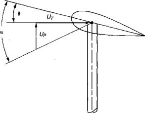
In order to define increments of lift and drag acting on a blade element in forward flight, it is necessary to write the equation for the angle of attack at the element as a function of the radial station and the azimuth position. For this analysis, it will be assumed that the rotor has no hinge offset and that flapping harmonics above the first may be neglected. The local angle of attack, shown in Figure 3.28, is made up of two angles just as it is in hover—the blade pitch and the inflow angle:
![]() a = 0 + tan-1
a = 0 + tan-1
4
The use of UT in this equation is based on the concept originally proved fdr swept wing airplanes—that only the velocity normal to the leading edge counts. The blade pitch has already been defined as a Fourier series:
f
9 = 0O + 0X — — Л, cosxj/ — Bx sin j/
К
and the equation for the tangential velocity, UT, has been derived:
UT = CtR I + |i sin у
The perpendicular velocity, Up, is a vector that is perpendicular to the blade quarter-chord line and lies in a plane that contains the rotor shaft. It is positive going up and consists of several components, as shown in Figure 3.29.
|
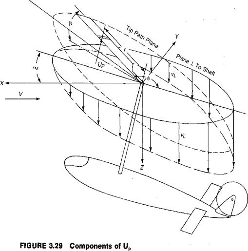
Up = Vas — vL — rp — Fp cos |/
A description of these components follows:
• F a—the component of forward speed that is parallel to the rotor shaft. (Note that a positive angle of attack is with the nose up, as shown in Figure 3.29, just as it is for airplanes. Helicopters generally fly nose down, or with negative angles of attack, but the sign convention was established when only autogiros—which do fly nose up—had rotors.)
• Vp—the local induced velocity, which for normal flight conditions may be considered to be parallel to the rotor shaft: For subsequent analysis, it will be convenient to use the angle of attack of the tip path plane as a reference angle rather than the angle of attack of the plane perpendicular to the shaft. Figure 3.30 shows the relationships between the various planes which are used in rotor analyses. Much of the early work, such as in references 3.16 and 3.17, used the control plane as a basic reference system. This is sometimes called the "plane of no feathering.” Later investigators for convenience have switched to the shaft plane or to the tip path plane—which is the "plane of no flapping”—as their basic reference planes. From Figure 3.30, it may be seen that:
Ct; ~ ^TPP ~ ais
Rear View
FIGURE 3.30 Rotor Angle Relationships
If all angles—including un~l(vJflR)—are expressed in degrees, then a is also in degrees. Note that when a is expressed in this form, the combinations of cyclic pitch and flapping, (Al — bj and (Bt + atJ, occur as primary variables. This is a consequence of the equivalence of flapping and feathering, which says that as far as rotor aerodynamics are concerned, one degree of cyclic pitch produces the same effect as one degree of flapping. (This equivalence strictly applies only to rotors with zero flapping hinge offset, but it is a good assumption for the analysis of performance of rotors that have moderate flapping hinge offsets or even for hingeless rotors which flap through structural bending. For analysis of stability and control, the hinge offset is significant and is discussed in Chapter 7.) In some of the early rotor analyses, such as in reference 3.17, these combinations of cyclic pitch and flapping are referred to as flapping with respect to the "plane of no feathering” and are designated ax and bx
a — + as
K = -(Ax-bx)
The equation for the local angle of attack contains several types of quantities that are either known or which may be computed: [3]
• |i, tip speed ratio = V/ClR.
• 0-rpp, angle of attack of the tip path plane required to put rotor thrust, helicopter weight, and helicopter drag into equilibrium.
• a0, coning of blades, which is established by equilibrium between lift and centrifugal forces.
• vJClR, induced velocity ratio, where vx is from momentum equation.
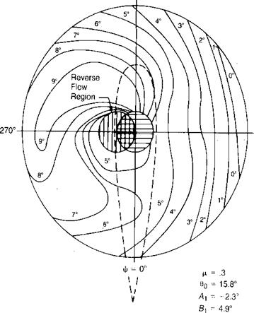
The flight conditions for the example helicopter have been determined at a tip speed ratio of 0.3 (115 knots) by methods to be outlined later, and the resultant angle of attack distribution has been plotted in Figure 3.31. Note that the angle of attack of the advancing tip is in the neighborhood of 0°, while the retreating tip is nearly 10°. The angle of attack on each side of the boundary of the reverse flow region goes to ± 90°, but since the local velocity is zero along this boundary, these high angles have little practical significance.
|
Ф = 180°
otjpp – -3.7° Cjla = .086 |
CLOSED-FORM EQUATIONS
Again, just as in hover, there are two schemes for integrating the forces on the blade elements to give rotor performance. The first method involves performing the integration of the equations mathematically to produce closed-form equations as a function of rotor geometry and flight conditions. The second method, suitable for a computer, performs the integrations by numerical methods. The closed-form integration method produces equations that are useful for rough calculations and for giving an understanding of the important factors; but since it must use simplifying assumptions in order to make the integration feasible, accuracy is sacrificed for convenience. The numerical integration method, which will be outlined later, uses a minimum of assumptions so that the resulting accuracy is high, but it is inconvenient without investing considerable time and effort in programming and checking out the computer.
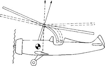
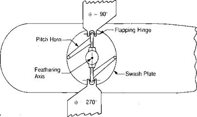
In the early Cierva autogiros, the rotor was simply a lifting device and roll and pitch control were obtained by ailerons on stub wings and by a conventional elevator, neither of which was very effective at low speed. Following his early successes, Cierva developed a means of obtaining direct control by tilting the rotor on a gimbal with respect to the shaft. With this scheme, pitch and roll control were generated by tilting the rotor thrust vector to give it a moment arm with respect to the center of gravity, as shown in Figure 3.26. This allowed Cierva to do away with the airplane control surfaces, but as autogiros became larger the control forces required to tilt the rotor became so high that flight was difficult. At this point, a means of rotor control called cyclic pitch was developed. In this system— which is almost universally used at present—the pilot cyclically changes the pitch of the blades about feathering bearings by tilting a mechanism known as a swash – plate. A schematic of this system is shown in Figure 3-27. It may be seen that if the swashplate is perpendicular to the rotor shaft, the blade angle is constant around the. azimuth, but that if the swashplate is tilted, the blade pitch will go through one complete feathering cycle each revolution. If the pilot pushes the stick forward, the swashplate is tilted forward. Since the pitch horn from the blade is attached to the swashplate 90° ahead, the blade has its pitch reduced when it is on the right side and has its pitch increased when it is on the left side. When the blade is over the nose or the tail, the forward tilt of the swashplate has no effect on the blade pitch.
Cyclic pitch can be used for two purposes: to trim the tip path plane with respect to the mast, and to produce control moments for maneuvering. In the first case, the pilot can mechanically change the angle of attack of the blades by the same amount as the flapping motion would have, thus eliminating the flapping. This can be used to eliminate all of the flapping or to leave just enough to balance pitching or rolling moments on the aircraft such as those due to an offset center of gravity.
|
T T
FIGURE 3.26 Pitch Control by Direct Rotor Tilt |
|
Thrust |
|
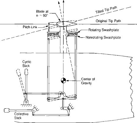
FIGURE 3.27 Schematic of Swashplate Control System |
In the second case, the pilot deliberately introduces an unbalanced lift distribution in order to make the rotor tilt for maneuvering. For example, if the helicopter is hovering and the pilot wishes to tilt the nose down, he pushes the stick forward, which tilts the swashplate down in front. The pitch of the blade at ф = 90° is decreased and that at ф = 270° is increased. The resultant imbalance accelerates the right-hand blade down and the left-hand blade up. The rotor flaps down over the nose and up over the tail, tilting the rotor thrust vector forward to produce a nose down pitching moment about the center of gravity, as shown in Figure 3.27. The procedure is similar if the pilot wishes to pitch nose up or to roll in either direction. Whether being used for trim or for control, the cyclic pitch is equivalent to flapping in that the changes in rotor conditions due to one degree of cyclic pitch are the same as those due to a one-degree change in flapping. Like the flapping, the blade pitch can be written’ in terms of a Fourier series:
0 = 0O + —- 0t — Ax cos у — Bx sin у К
where 0O is the average pitch at the center of rotation, 0t is linear twist, Ax is half the difference in pitch between the blade over the tail and the blade over the nose, taken as positive when the pitch at у = 180° is larger. Bx is half the difference in pitch between the advancing and retreating blades, taken as positive when the pitch on the retreating blade is gfeater than the pitch on the advancing blade. The coefficient, Ax, is called the lateral cyclic pitch because it is used by the pilot to produce rolling motion, and Bx is called longitudinal cyclic pitch because it is used to produce pitching motions. (This nomenclature is based on the results as the pilot sees them rather than on the geometry of the control system as seen by the designer.)
The use of cyclic pitch for trim makes it possible to eliminate the flapping hinges in the so-called rigid rotor designs. If a fully articulated rotor were trimmed with cyclic pitch so that the tip path plane was perpendicular to the rotor shaft, then it would be possible to freeze the flapping hinges with no change in the rotor condition, since there was no motion about the flapping hinges in the first place. Thus the flapping rotor with cyclic pitch could be converted into a rigid rotor with cyclic pitch. Similarly, if a rigid rotor were trimmed with cyclic pitch such that there were no cyclic flapping moments in the blade roots, then hinges could be introduced with no effect on the flight conditions. Thus the rigid rotor with cyclic pitch could be converted into an articulated rotor with cyclic pitch. From this, it may be seen that for the totor trimmed perpendicular to the mast, or nearly so, there is no essential difference between an articulated rotor and a rigid rotor. Where differences do exist will be discussed in Chapter 7.
Besides cyclic control, which the pilot obtains by tilting the swashplate with the cyclic stick held in his right hand, he has also the collective control that changes the pitch of all blades simultaneously by raising and lowering the entire swashplate. This is done with the collective stick, as shown in Figure 3.27.
In order to develop equations for the angle of attack of the blade element, it is necessary to understand the blade motion known as flapping.
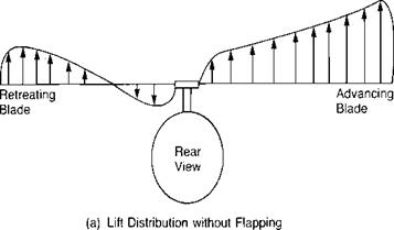
During the early development of the autogiro, Juan de la Cierva tried to obtain structural integrity for his rotor by bracing the blades with landing and flying wires just as the wings of airplanes were braced in those days. On the first attempted takeoff, the aircraft rolled over on its side and smashed the rotor before it had attained flying speed. Cierva rebuilt the machine, but on the next takeoff it again rolled over and smashed the rotor before it had attained flying speed. This action was a mystery to Cierva, since he had flown a rubber-powered model autogiro and had observed no appreciable rolling moment. The model had been built with rattan blade spars and since, in model size, this type of construction was structurally adequate, there was no need for the landing and flying wires that he used on his full-scale rotors. After much thought, Cierva realized that it was the difference between the rigid, wire-braced rotor of the full-scale aircraft and the flexible blades of the model rotor that accounted for the difference in rolling moment. It has already been pointed out that in forward flight, the advancing blade has higher velocities acting on it than the retreating blade. If each blade had the same pitch setting, their angles of attack would be nearly the same, but the difference in velocity would produce more lift on the advancing side than on the retreating side. This would produce an unbalanced rolling moment, as shown in
|
|
|
|
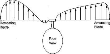
(b) Lift Distribution with Flapping
FIGURE 3.15 Effect of Blade Flapping on Lateral Lift Distribution
Figure 3.15a, which would be expected to roll the aircraft over. On the model, however, because of the flexibility of the rattan blade spars, the blades could bend up and down. Thus the advancing blade, which initially had high lift, began to accelerate upward. As it was accelerating upward, it was also being rotated toward the nose, where the local velocity was reduced to its mean value, so that no unbalanced lift existed and the blade stopped accelerating. The retreating blade was undergoing a similar experience except that it was accelerating downward as it rotated to a position over the tail. The flapping produced a climbing condition on the advancing blade as shown in Figure 3.16 and thus decreased its angle of attack. The retreating blade, on the other hand, was descending and thus experiencing an increased angle of attack. The rotor came to a flapping equilibrium when the local changes in angle of attack were just sufficient to compensate for the local changes in dynamic pressure. In this equilibrium condition, the rotor was not tilted sideways but was tilted fore and aft as shown in Figure 3.17, and the lift distribution was balanced as shown in Figure 3.15b rather than unbalanced as in Figure 3.15a.
|
|
|
FIGURE 3.16 Change in Angle of Attack Due to Flapping |
|
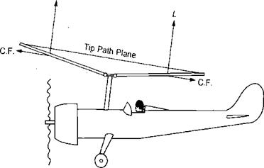
FIGURE 3.17 Autogiro in Level Flight |
When this phenomenon became clear to Cierva, he knew what he had to do: add flexibility to his full-sale rotor. He decided that the simplest solution would be to use a mechanical hinge that would allow the blades to flap and automatically eliminate the rolling moment that had given him such serious problems. The only wires retained were those used to prevent the blades from flapping down too far as the rotor was stopped. In flight, the blades were kept extended by a combination of lift and centrifugal forces, as in Figure 3.17. When such a rotor is established in its stable flapping position, there are no accelerating forces on it causing it to flap with respect to an axis system fixed in the tip path plane. Thus in order that the moments at the hinges are zero, the aerodynamic moment must be a constant around the azimuth and numerically equal to the centrifugal force moment produced by the coning, which is also a constant since the tip path is assumed to lie in a plane. Any change in the distribution of the aerodynamic moments due to changes in flight conditions will force the rotor to seek a new stable flapping position where the aerodynamic and centrifugal moments will again be constant, equal, and opposite around the azimuth.
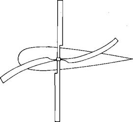
With this technological breakthrough, Cierva was able to fly his autogiro and began a long line of development that has resulted in most present-day helicopters having rotors with flapping hinges. The invention of the flapping hinges did not cure ail of Cierva’s rotor problems, however. He was plagued with high stresses and structural failures in his early blades resulting from moments in the plane of the rotor disc, the so-called inplane moments. These were due to a combination of cyclically varying drag and inertia (or Coriolis) loads. The drag variation was caused by the previously discussed nonuniform aerodynamic environment in which even though the blade lift was made uniform around the azimuth by flapping, the drag was not. The nonuniform inertial loads were the result of the blades obeying a physical law called the law of conservation of momentum, whose effects are familiar to those old enough to remember the swiveling piano stool and the trick of holding a pair of heavy books at arm’s length while being set spinning by a friend. As the books were pulled in toward the body, the spin became faster and faster. The same principle is used by a figure skater to produce a highspeed spin. The law of conservation of momentum states that the product of the moment of inertia and the rate of spin is a constant. As the blade flaps up, its center of gravity moves in toward the spin axis, as shown in Figure 3.18. The same thing happens for the down-flapping blade. This reduces the moment of inertia so each blade tries to speed up. If they are resisted by the inertia of other blades, they will try to bend forward, thus producing inplane bending moments and corresponding stresses in the blade roots. Note that each blade of flapping rotor goes through this cycle twice in a revolution, thus producing two-per-rev—-or 2 P—stresses. Had Cierva’s rotor had only two blades, these stresses would have been minimized since the blades would have acted in unison with nothing to restrain them. As it was, Cierva’s rotor had four blades, and it had problems. He decided that if one hinge in a blade was good, two must be better; so he incorporated vertial hinges such that the blades could move back and forth in the plane of the rotor without generating stresses in the roots. These hinges are now known as lead-lag hinges and, in conjunction with the flapping hinges, produce the
|
|
|
FIGURE 3.18 Inplane Blade Bending Due to Flapping Motion |
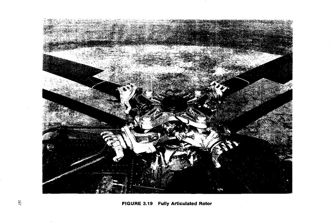
fully articulated rotor systems used on many helicopters today. The lead-lag hinges are important in the study of rotor loads, vibration, and such specialized problems as ground resonance; but they have no effect on performance, stability, or control. For this reason, they will be neglected in the remainder of this book.
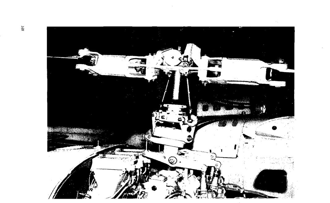
A fully articulated rotor is shown in Figure 3.19. Some designers have elected to put enough structure into the blades and hub that the inplane stresses can be kept to a low and safe level without lead-lag hinges as in the rotor of Figure 3.20 and some designers have even eliminated the flapping hinge by substituting a flexible section of the hub. This latter system is the so-called rigid rotor or hingeless rotor of Figure 3.21, which will later be shown to be equivalent to a hinged rotor with offset flapping hinges.
The 90° lag between the maximum aerodynamic input and the maximum flapping is typical of systems in resonance, and it may be shown that the rotor is a resonating system by the analogy of a mass supported on a spring, as shown in Figure 3.22. The mass will have a characteristic natural frequency at which it will oscillate if it is plucked and then released. The natural frequency will be equal to /k/m rad/sec. If, instead of plucking the mass, a variable-speed electric motor
|
|
|
FIGURE 3.20 Teetering Rotor |
|
|
![]() Hingeless Rotor
Hingeless Rotor
 with an unbalanced flywheel is used to excite it at various motor speeds, it will be found that the speed at which the motion of the mass is the greatest will be exactly the same as the natural frequency found by plucking the system. At this speed, it may be said that the mass is in resonance with the exciting frequency.
For a rotating system such as a rotor blade, the natural frequency is given by an equation similar to that for the spring and mass:
where К is the rate of the restoring moment about the flapping hinge in foot pounds per radian of flapping angle, and I is the moment of inertia of the blade about the flapping hinge. The restoring moment is due to the centrifugal force acting though a moment arm which is a function of the flapping angle, p, as shown in Figure 3.23. The centrifugal force acting on a blade element a distance r from the center of rotation is:
AC. F. = Cl2mAr
where m is the mass per running foot. The restoring moment due to this centrifugal force is thus:
AM = AC. F. rp or
AM = nv2wpAr
and the total restoring moment obtained by integration is:
Substituting this into the equation for the natural frequency gives:
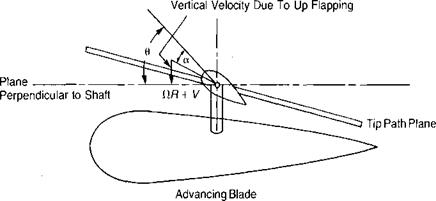
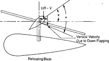
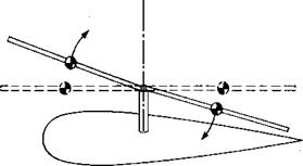
This says that the natural frequency of the flapping motion of a blade is equal to its rotational speed no matter what that speed is, and that the blade will always be in resonance with the exciting forces caused by the once-per-revolution unbalance of the aerodynamic forces. (Strictly speaking, this is true only for a blade without hinge offset, but it is nearly true for all blades. See Chapter 7 for the effects of offset.) The blade in resonance will exhibit the characteristic 90° lag between input and response that is inherent in all resonating systems. The result is that the rotor flaps fore and aft rather than laterally in response to unequal dynamic pressure on the advancing and retreating blades. In addition, a small amount of lateral flapping will be generated due to another aerodynamic effect. As the rotor
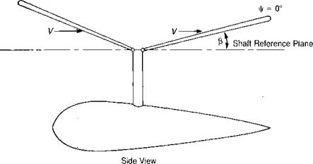
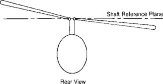
produces lift, it is coned by the combination of lift and centrifugal forces. In forward flight the blade over the nose experiences air coming toward its lower surface, whereas the blade over the tail experiences air approaching it from on top, as shown in Figure 3.24. The result is that the angle of attack on the blade at у = 180° is increased and the angle of attack of the blade at V|/ = 0° is decreased. The rotor compensates for this inequality in the same manner as it did for the nonsymmetric velocity patterns on the advancing and retreating blades: it responds 90° later by tilting up on the retreating side and down on the advancing side. This causes flapping velocities over the nose and over the tail that are exactly enough to compensate for the difference in angle of attack caused by the coning.
The flapping motion may be represented by an infinite Fourier series:
(3 = a0 — als cosvj/ — bls sin vj/ — als cos 2^ — b2s sin 2|/ • • • — и cos — b„s sin n\f
(where j/ is as defined in Figure 3.14.)
|
|
|
FIGURE 3.24 Velocity Orientation Causing Lateral Rotor Tilt |
Only the first three terms will be used in the subsequent analysis since it may be shown using the equations of reference 3.15 that the second and higher harmonics represented by the remaining terms are relatively small and have very little effect on rotor thrust ancj torque. Thus it will be assumed that:
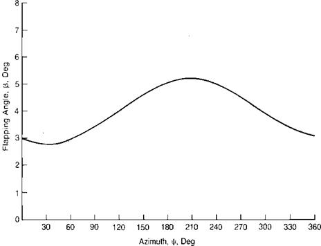
P = a0 — ax^ cos |/ — bls sin |f
where aQ represents the average value, or coning; aXj is the longitudinal flapping with respect to a plane perpendicular to the shaft defined as positive when the blade flaps down at the tail and up at the nose, and bx is the lateral flapping defined as positive when the blade flaps down on the advancing side and up on the retreating side—the normal condition. For the flapping shown in Figure 3.25, the coefficients are:
я0 = 4.0 ax = 1.0
lS
bx =0.5
lS
|
FIGURE 3.25 Typical Flapping Angle Response |
Just as in hovering, the momentum, or energy, method is useful in understanding the physics of forward flight and for making rough calculations; but the blade element theory must be used to define flight limitations and to do more accurate calculations. In forward flight, the velocity acting on the blade element is a function of both the radial station and the blade azimuth position.
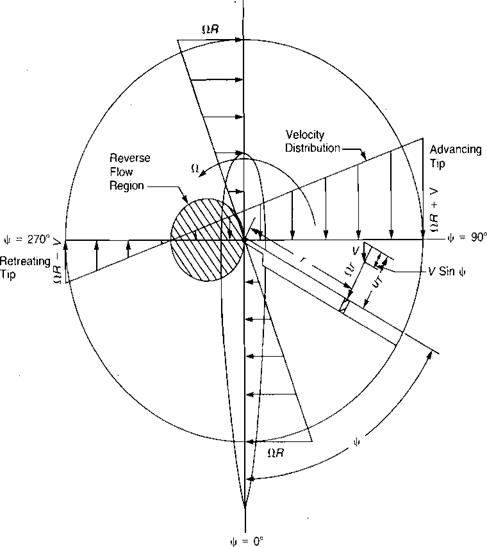
The azimuth angle, |/, is defined as shown in Figure 3.14 with |/ = 0 over the tail. The velocity acting on the blade element is the vector sum of the velocity due to rotation, fIr, and the forward speed of the helicopter, V. The study of swept – wing aerodynamics has shown that the component of velocity perpendicular to the leading edge is the only velocity that is important in establishing aerodynamic forces. The velocity perpendicular to the leading edge—or tangential to the chord of the element—UT, is:
Uf = Clr + Fsin|/
|
V »|i = 18Gr
FIGURE 3.14 Tangential Velocities in Forward Flight |
Over the tail and over the nose, the blade element sees the same velocity as it would in hover, but on the advancing blade it sees a higher velocity, and on the retreating blade a lower. As a matter of fact, on the retreating blade there are elements where the velocity perpendicular to the leading edge is actually negative—that is, air strikes the trailing edge rather than the leading edge of the blade. Figure 3.14 shows the vector addition of the velocities for the blades at the cardinal azimuth positions. If the equation for UT is set to zero, the radius station at which the velocity vanishes is:
![]() sin |/
sin |/
A plot of this relationship is a circle that is tangent to the rotor centerline. Inside this circle, UT is negative, and the zone is called the reverse flow region.
Using the definition of the tip speed ratio, Ji, the equation for the tangential velocity may now be written:
UT = flR — + p sin j/
V R /
Energy methods based on the power required in level flight are useful for making first approximations of the extra power required to climb or the rate of descent in
|
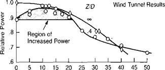
ZJD
Forward Speed, knots |
|
Forward Speed, knots FIGURE 3.11 Experimental Evidence of Ground Effect |
Sources: Cheesman & Bennett, “The Effect of the Ground on a Helicopter Rotor in Forward Flight,” British R&M 3021, 1957; Sheridan & Wiesner, “Aerodynamics of Helicopter Flight Near the Ground,” AHS 33rd Forum, 1977.
autorotation. For more exact calculations, the methods outlined in the section on use of the charts later in this chapter should be used.
The extra power required to climb compared to that required to fly level may be estimated from the rate of change in potential energy. For a rate of climb, R/C, in ft/min:

(R/C)(GM.)
33,000
For the example helicopter this approach gives a first approximation:
Ah. p.dimb = Q.6l(R/C)
The best rate of climb will be achieved at the speed for which the power required for level flight is a minimum, since at this speed the A h. p. available from
the engine will be a maximum. Figure 3.8 shows that for the example helicopter this speed is about 75 knots.
In autorotation, the same approach may be used; that is, the rate of change of potential energy must be large enough to supply power equal to that required for level flight:
 33,000 h. p.
G. W.
The minimum rate of descent also is achieved at the speed for minimum power required in level flight. The effect of several significant parameters on the autorotative rate of descent can be seen by writing the power-required equation as:
Thus:
The effect of varying disc loading, equivalent flat plate area, and gross weight on the autorotative rate of descent of the example helicopter at 75 knots is shown below. (The profile power is assumed to remain constant).
|
Case Parameter |
One |
Two |
Three |
Four |
Five |
|
Disc loading, D. L. |
7.1 |
3.55 |
7.1 |
3.55 |
7.1 |
|
Equiv. flat plate area,/ ft2 |
19.3 |
19.3 |
19.3 |
19.3 |
9.65 |
|
Gross weight, G. W. |
20,000 |
20,000 |
10,000 |
10,000 |
20,000 |
|
h. p., level flight |
. 1,070 |
780 |
780 |
635 |
1,025 |
|
K/DAuto> ft/min |
1,765 |
1,295 |
2,580 |
2,100 |
1,690 |
Comparing cases 1 and 4 leads to the somewhat surprising conclusion that the lighter a helicopter, the faster its autorotative rate of descent. This paradox can be explained by comparing the total potential energy at the two weights and the power required to fly in level flight. The potential energy is only half as much in case 4 as in case 1, but the power required is more than half as high. To obtain this power from the loss in potential energy, the lighter helicopter must come down faster.
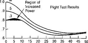
Figure 3.13 shows results obtained during flight tests of the Lockheed Model 286 helicopter. The decrease in rate of descent with increasing gross weight
 |
Source: Internal Lockheed report.
is evident. The trend would be expected to hold only until the rotor was so heavily loaded that blade stall- would cause the profile power to increase rapidly.