Category Helicopter Performance, Stability, and Control

The lift of a rotor blade—or of a wing—goes to zero at the extreme tip, but it starts falling off some distance inboard. Thus the integration of the equation for rotor lift to the extreme tip is somewhat optimistic. A similar optimism, though of somewhat lesser importance, is introduced by’ starting the integration at the center of the rotor even though the blade "cutout” may be 10% to 25% of the radius. Figure 1.16 shows the theoretical and realistic lift distributions for a blade with

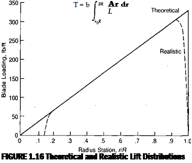ideal twist. A numerical method for computing the shape of the lift distribution at the tip has been developed for propeller analysis and adapted for rotors in Reference 1.3. This method, known as the Goldstein-Lock method, is sometimes incorporated in digital computer hover performance programs. A more convenient scheme, however, is to use modified limits of integration such that:

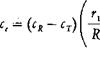
where x0 is the fraction of root cutout and BR is the effective outer radius, which is picked such that the area under the theoretical lift distribution out to BR is the same as the area under the actual curve out to JR. The amount of the tip loss is dependent on the total lift of the blade and its geometry. The higher the lift, and the wider the chord with respect to the radius, the further inboard the lift starts falling off. Both these effects are included in an empirical equation for В that was first derived by Prandtl and gives satisfactory correlation with the Goldstein-Lock calculations for lightly loaded rotors.

[гс~т

b

For the main rotor of the example helicopter hovering at sea level, the equation gives an effective radius factor, B, of 0.97.

When root and tip losses are accounted for, the momentum equations previously derived should be modified. This can be done by defining an effective disc loading, D. L.cff, based on the effective disc area, which is smaller than the true area:

Thus:

For the example helicopter,

D. L. = 7.1 lb/ft2

But

Thus at sea level

vle((= l4.5y/lJ = 40.2 ft/sec

instead of the 39 ft/sec previously calculated.

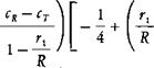
With root and tip losses accounted for, the equation for Ct/g becomes:

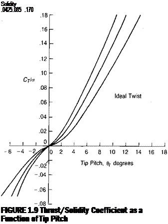
CT/o=(B2 —*^(Є, — ф,)

The value of the induced angle, ф„ now must be based on only the effective disc area, although the definitions of the nondimensional coefficients are still based on the geometric rotor radius. Thus ф, becomes:

CT

2 (B2-xl)

gCj/g

Solving the equation for Ct/g gives for pitch at the blade tip, 0;:

For the example helicopter with an ideally twisted rotor, the tip pitch required at the design hover condition is 7.1° instead of the 6.7° calculated. without the losses. Since the lift falls off toward the tip, the induced drag also falls off, but the profile drag does not. At the root, there may not be any lifting surface, but there is always a spar or a section of the hub that has drag even if it has no lift. Thus the profile drag must be integrated from root to tip. Considering the increased inflow angle due to the decrease in effective disc area, the expression for Cp/a of a rotor with ideal twist is:

aCr/a cd 2 (B2-xi) +~8

The drag coefficient for use in this equation should be found from airfoil data such as in Figure 1.10 and an average angle of attack, which is:

_ 57.3Ct/g

CL =- ;—- V

B2-x20

For the example helicopter with ideal twist, this method gives the rotor power required for hover at the design gross weight as 1,840 horsepower if root and tip losses are not considered and 1,900 horsepower if they are, a difference of about 3.2%.

There is no easy way to verify experimentally the simple hover tip loss equation, but it may at least be partially justified by comparing the results of hover calculations made using it with those made using the more sophisticated prescribed wake vortex method. Figure 1.17 shows the calculated ideal Figure of Merit, assuming no profile drag, as it is affected by number of blades. The solid line is from reference 1.2 and was calculated for uniform inflow using a prescribed wake vortex method. The dashed line is for a rotor with ideal twist and is based on the reduction of disc area due to root and tip losses and also includes the effect of wake rotation, as discussed in a later section. It may be seen that the shape of the two lines is essentially the same, indicating that the simple tip loss equation is in good company.

A blade—whether hinged or cantilevered from the hub—seeks an equilibrium coning angle that is a function of the lift, centrifugal forces, and blade weight. The magnitude of the coning, a0) may be found by setting the moments at the hinge— or at the effective hinge—to zero:

^hingc = Afjift + Mcf + Mw — 0

For most engineering calculations of coning, it is sufficiently accurate to assume that the hinge is at the center of rotation. In this case, the moment due to lift is:

UL, — rdr

dr or for a blade with ideal twist:

Mlift = f – CL2Rac(Qt – ф,)гУг = – —Cl2pacR4

l 2 ‘ 3 a

The moment due to centrifugal force is:

where m is the mass per running foot and Ih is the blade’s moment of inertia about its flapping hinge. (It can be assumed to be equal to the rotor’s moment of inertia divided by the number of blades.)

Setting the sum of the three moments equal to zero and solving for a0 gives:

The combination of terms, pacR*/Ih is a nondimensional parameter, y, known as the Lock number after a pioneer British autogiro aerodynamicist, C. N. H. Lock. It represents the ratio of aerodynamic to centrifugal forces. Two blades that have the same airfoil and aspect ratio, and are constructed of material with the same density, will have the same Lock number no matter what their radius. The heavier the blade, the lower the Lock number. For operational blades, it varies from 10 for lightly built blades to 2 for blades of tip-driven helicopters with concentrated masses at the tips. The rotor parameters for the example helicopter are given in Appendix A. From these values:

The last term in the equation for coning is the contribution of the dead weight of the blade where:

= – gmrdr

If the blade has a uniform mass distribution, then:

X–W‘

and the coning equation may be written:

2 CT/a 2gR

As a general rule, the weight contribution is negligible except for very large rotors. For the example helicopter at its hover conditions; the calculated coning is 4.4° if the last term is ignored and 4.3° if it is included.

Although the derivation of the equation for coning was based on the assumption of a blade with a flapping hinge, it is also valid for flexible blades cantilevered from the shaft without hinges since the aerodynamic and centrifugal forces overpower whatever structural stiffness the blades might have.

Some past analyses have mistakenly led to the conclusion that there is an upper limit to how big a rotor can be built because of excessive coning. That this is an erroneous conclusion is evident from the foregoing equation provided the Lock number, y, and the blade loading coefficient, CT/a, are constants. As a matter of fact, the coning will actually decrease because of the weight term as radius is increased while holding the same tip speed.

The equation provides a simple method of estimating the maximum coning that a rotor can develop. Earlier it was shown that CT/o is approximately 1/6 of the average lift coefficient, ct. Assuming a maximum value of 1.2 for this parameter gives a maximum value of 0.2 for CT/o. Later discussions will show that this is a reasonable upper limit. For the example helicopter with a blade Lock number of 8.1, this results in a maximum coning of just over 10°.

Review of Assumptions

The discussion of hover performance up to this point has been based on a number of simplifying assumptions. For normal rotors in normal flight conditions, the use of these assumptions gives good results consistent with a first approximation method; but when more accuracy is required, the assumptions must be challenged and their effects evaluated. The most important of the assumptions are:

• Assumption: The lifting portion of the blade extends from the center of rotation to the extreme tip.

Challenge: The lifting portion of the blade actually starts sonle distance outboard from the center, and the tips are only partially effective.

• Assumption: Induced velocities are uniform over the disc.

Challenge: Induced velocities are nonuniform.

• Assumption: The blades have ideal twist.

Challenge: No actual blades have ideal twist.

• Assumption: The blades are rigid torsionally so that no structural twisting takes place.

Challenge: No blade is infinitely rigid, and a rotating blade is subjected to twisting moments from several sources.

• Assumption: Blades have constant chord.

Challenge: Some blades are tapered.

• Assumption: The wake does not rotate.

Challenge: The wake does rotate.

• Assumption: There is no effect of tip vortices on the angle of attack of a following blade.

Challenge: Tip vortex interference has been found to be significant.

• Assumption: The airfoil lift and drag characteristics are the same as the NACA 0012 characteristics of Figure 1.10.

Challenge: Many rotors use airfoils different than the NACA 0012.

• Assumption: The airfoil characteristics are not a function of local stall or compressibility effects.

Challenge: Stall and compressibility effects impose significant power penalties in some flight conditions.

• Assumption: There are no effects due to radial flow.

Challenge: There are some effects due to radial flow.

• Assumption: The rotor is far from the ground.

Challenge: In some cases the rotor is close to the ground.

Some of these assumptions result in errors in the calculation of the hover performance; others are good assumptions in that their consequences are negligible. In order to differentiate between the two types, the assumptions will be discussed one at a time.

On most helicopters, the critical design condition is high-speed flight. To satisfy this condition, the twist is usually less, and the blade area usually more than is

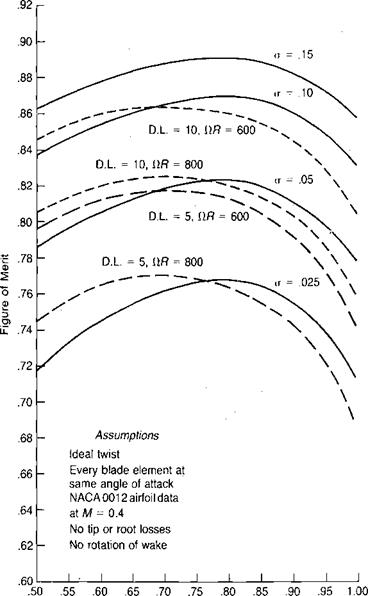
optimum for maximum hovering performance. On some helicopters, such as flying cranes, however, the rotor may be designed by the hover requirement. For these cases, it is well to have an understanding of the maximum theoretical value of the Figure of Merit and how it varies with rotor parameters.

For a rotor with ideal twist, the Figure of Merit may be written in terms of nondimensional coefficients:

Induced power C pi С Ty CT/ 2

F. M. =———————– = — – ——————————

Actual power Ct Ст^Д+с_^

It may be seen that if the rotor had neither drag nor solidity, the Figure of Merit would be unity. Since neither condition applies to actual rotors, the Figure of Merit will always be less than unity. Using the relationship:

The Figure of Merit becomes:

This form of the equation shows that the Figure of Merit is highest for high solidities and for high values of cbl2lcd. (Note: Sailplanes have their lowest rates of sink when their values of C[/2/CD are at a maximum.) The equation represents the theoretical maximum Figure of Merit for a rotor with ideal twist, no tip or root losses, and with every blade element operating at the same angle of attack. This theoretical maximum has been compared with whirl tower results in Figure 1.12. The whirl tower Figure of Merit is from reference 1.1 and the theoretical curve is based on the NACA 0012 airfoil data of Figure 1.10, which are from the same set of tests. The difference between the two curves is due to tip and root losses, nonideal twist, nonuniform blade element angles of attack, and rotation of the wake (all of which will be discussed before we finish).

The equation for Figure of Merit can also be written as a function of disc loading and tip speed:

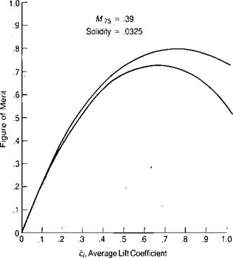
This form shows that for a given disc loading and tip speed, the Figure of Merit is maximum when cl]cd is a maximum. The apparent conflict with the previous discussion is sometimes called a paradox, but the truth of both statements is shown in Figure 1.13 on which the theoretical Figure of Merit based on the NACA 0012 airfoil data of Figure 1.10 has been plotted as a function of ct for both constant solidities and constant disc loadings. It may be seen that the curves for constant solidity peak at a ct of 0.8, which is the lift coefficient for maximum c)/2/cd, and that the curves for constant disc loading peak at a ct of 0.7, which is the lift coefficient for maximum cjcd. It should be noted that the constant disc loading lines are a function of tip speed; the lower the tip speed, the higher the potential Figure of Merit. The benefit, of course, is decreased if the higher solidity required by the lower tip speed requires higher blade weight. The equation leads us to conclusions that can also be obtained graphically, as presented in Figure 1.14. This shows the velocities and forces acting at a typical blade element of three rotors developing the same thrust. The first rotor is the baseline. The second has half the diameter resulting in four times the disc loading, which doubles the induced velocity and thus the induced drag. Since the lift-to-drag ratio is assumed to be the same, the profile drag is the same. The Figure of Merit is proportional to the induced drag

FIGURE І.13 Calculated Figure of Merit

divided by the sum of induced drag and profile drag. At the higher disc loading, this ratio is closer to 1.0 than for the baseline rotor. This explains why designers of high disc loading aircraft can claim a higher Figure of Merit than can designers of low disc loading aircraft. The third rotor has the same diameter as the baseline but only half the tip speed. The lift vector is tilted further back, leading to twice the induced drag and to a similar increase in Figure of Merit as for the second rotor. It should be noted, however, that whereas the high disc loading rotor takes almost

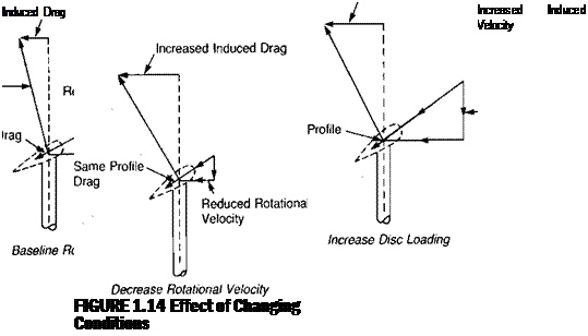
twice the power of the baseline, the low tip speed rotor requires about the same since the power is proportional to the product of drag and speed.

Another study of the maximum figure of Merit is given in reference 1.2. Figure 1.15 presents the results for a four-bladed rotor with constant induced velocity as the maximum attainable Figure of Merit versus thrust coefficient. The top line is the Figure of Merit assuming no drag. It is unity only for zero thrust. At higher values, wake swirl and tip vortex interactions (to be discussed later) combine to produce some unavoidable losses. The lower lines show how drag affects the results. The drag characteristics assumed for this study were simply based on skin friction as a function of Reynolds number but independent of angle of attack and Mach number as expressed by the equation:

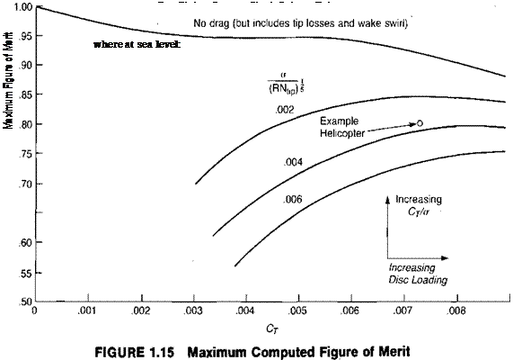
R. N. = 6,400 cV

The family of lines essentially represents constant values of rotor solidity. Going down in solidity (up in CT/d) increases the maximum Figure of Merit. For constant solidity, increasing disc loading or decreasing tip speed increases CT and thus the Figure of Merit. In any case, the study indicates the maximum optimistic hover performance. The calculated value for the Figure of Merit for the example helicopter is shown as a point at about 0.80.

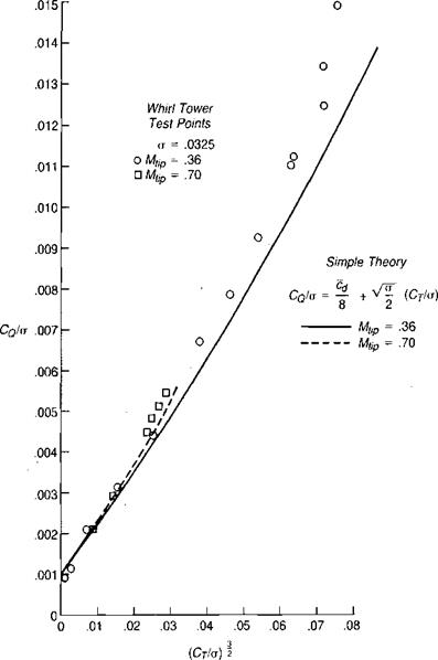
The torque equation can be used to plot Cq versus CT—or, more conveniently, Cq/g versus CT/a, where:

C(/(T = Cp/a = у® (CT/a)}/’ + – j

The derivation of this equation has been based on ideal twist and a number of other simplifying assumptions and thus should not be used uncritically to compute the performance of all rotors. It does, however, provide a guide to interpreting actual performance data such as Figure 1.11, where Cq/g has been plotted against (CT/o)i/2 for whirl tower data from Reference 1.1. The theoretical line is based on the value of ~cd determined from Figure 1.10 as a function of the average angle of attack and the Mach number at the 75% radius. It may be seen that although there

is some discrepancy between the theory and the test points, the general characteristics of the theoretical line are the same as the test results. The reasons for the discrepancies that do exist will be discussed in a later section.

The average value of the drag coefficient, cd, for use in the anajy^, obtained by using an average value of angle of attack and the corresp^ ls may ^ coefficient as determined by wind tunnel tests of two-dimensional ai^f ^ing Figure 1.10 shows the characteristics of the NACA 0012 airfoil sectl^ Actions typical of the airfoils actually used on blades. These characteristics hav^ ?> Miich is from reference 1.1 and were synthesized from whirl tower tests of taken rotor over a wide range of collective pitch and tip speed by choosing * c°mplete drag coefficients that brought the test results into the best agreeing lift arJ theory. The results of two-dimensional wind tunnel tests of the same ^ Mth the used as a guide. Figure 1.10 shows the lift and drag coefficients as

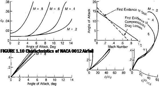
^ions of

both the angle of attack and the Mach number. Also shown are other characteristics of importance to the helicopter aerodynamicist, which will be discussed later. The average lift coefficient for the rotor, is:

Сі — ай

But it was shown earlier that

cі ——

therefore,

6CT/o

a =———–

a

If it is assumed that the slope of the lift curve is equal to 6 per radian,

then:

a = Су/a radians

or

a = 57.3 C/ /a degrees

For the example helicopter at sea level, the value of Ct/g is 0.086, and thus the average angle of attack is 4.9°. The Mach number at the 75% radius station— which may be considered typical of the entire blade—is 0.43. From Figure 1.10, the corresponding value of the drag coefficient is about 0.010.

The total torque can be obtained by integration in the same way that the total lift was:

R2a I (0, – ф,)фtrdr + cd I r’dr

a cd

-(0,-<МФ.+ —

2 4

Using expressions already derived, this becomes:

CT cdo

СЄ = Ст J~2+~tT

The first term in this equation is due to the combined effect of the rearward tilt of the incremental lift vectors in Figure 1.6 and is known as the induced torque coefficient. The induced torque coefficient could have been derived from the momentum equation by noting that the induced power is:

Pj = = T

and since it was earlier shown that CP was numerically equal to CQ:

CQi — Cp.= CT

This shows that the momentum theory and the blade element theory—at least for ideally twisted blades—produce the same expression for induced power. The second term in the equation for CQ is the profile torque coefficient and is due only to the drag of the blade elements. The Figure of Merit written in nondimensional terms is:

C„ CT/CJ2 _ fa (Cr/o)>n Cp C, – yj 2 Cs/c

The determination of rotor thrust as a function of blade angle is of some importance, but more important is the answer to the question, "How much power is required to produce the thrust?” The first approximation of the power required is obtained using the Figure of Merit method described earlier. The second approximation may be made with the blade element theory.

The increment of power, A P, produced by a blade element, is:

AP = AQfl

where the incremental torque, AQ, is equal to the drag on the blade element times the radius of the element. Just as for airplanes, the drag is made up of two parts: induced and profile. From Figure 1.6, it may be seen that since the lift is perpendicular to the local velocity, it is tilted back by the induced angle, ф. Thus the induced drag due to lift, ДЦ, is:

AD, = ДТф

The profile drag, AD0, is the force parallel to the local flow; and, since ф is considered to be a small angle, the component of profile drag contributing to torque is taken as being equal to the entire profile drag. Thus the increment of torque, AQ, is:

AQ = <Діф + Ad0)

The drag can be treated in the same way that lift was:

AD0 = ^(£ir)2cdcAr

where the drag coefficient, cd, may be considered a constant at this stage of the analysis.

The equation for incremental torque can now be written as:

^(Пг)2С/сАгф {Cir)2cdcAr

Expressions for Ci and ф for an ideally twisted blade have already been derived. Using these, the torque per running foot is:

The equation derived earlier for the thrust of a rotor with ideal twist can be written in nondimensional form:

the example helicopter and for solidities of half and twice this value are shown in Figure 1.9. For the example helicopter operating at a Cr/(J of.086, the required pitch at the tip is 6.7°. Note the relatively low slope of the curve near zero thrust. In this region, the induced velocity is important and a large amount of the blade pitch is used to compensate for it, with only a small proportion available to produce thrust. At higher values of thrust, the induced velocity is of less importance and more of the blade pitch is available to produce thrust.

The collective pitch of a blade with linear twist can be related to the tip pitch of a blade with ideal twist through the approximate relationship:

e„ = I e, -10,

Thus for the example helicopter with a linear twist of—10°, the collective pitch is approximately:

0 = I (6.7) – I (-10) = i7.6°

Before developing the analysis further, it is timely to introduce the concept of nondimensional coefficients. Just as does the airplane aerodynamicist, the helicopter aerodynamicist finds it convenient to work with nondimensional coefficients to define rotor characteristics in a form that is independent of rotor size. For this purpose, the system used by NASA will be adopted:.

рЛ(Ш)3

One of the convenient features of this set of coefficients is that the torque and power coefficients are numerically equal. This may be shown by writing the equation for power, P, in ft lb/sec as:

Substituting this into the equation for CP gives:

Note that the reference area for each of these rotor coefficients is the. rotor disc area, A. It is often desirable to use coefficients based on blade area rather than on disc area. In order to do this, the rotor solidity ratio, G, is defined:

Total blade area

G = ——- ■;————-

Disc area

As shown in Figure 1.8, the solidity is the amount of the rotor disc made solid by the blades:

Ab bcR be

A nP2 TR

For the example helicopter:

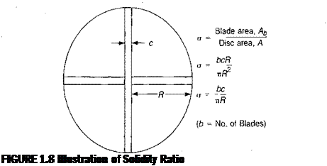120 (4)(2)

———- = ww- = 0.085

2,827 n(30)

Note that in using this definition, the blades are assumed to extend into the center of rotation where some overlapping of blade area occurs. This assumption is used in the definition of solidity even though, in practice, the actual blade sections do not start until some distance from the center of rotation. This is a satisfactory assumption since the inboard portions of the blades contribute little to the aerodynamic characteristics of the rotor. However, the same cannot be said about the outboard portions of the rotor. If the blade is tapered, the aerodynamic biasing toward the tips should be accounted for by rewriting the equation for solidity to define a thrust-weighted solidity as:

K_

nR

where

and c is the local chord.

For example, a blade planform might consist of a portion with a constant chord, cR, from the root to a point, rXi and then taper linearly to a tip chord of cT. The equation for the effective thrust weighted chord in this case is:

The rotor coefficients based on effective blade area are:

An analogy with airplane aerodynamics is that CT corresponds to span loading and governs induced power. On the other hand, CT/c corresponds to lift coefficient, and its value is used to determine the margin to blade stall just as CL is compared to

CLmix – The numerical value of CT/o may be related to an average two-dimensional lift coefficient,?/, by defining the lift per running foot as a function of the average lift coefficient, which for this purpose will be assumed to be constant along the blade:

AL

a7

Integrating out the blade and multiplying by the number of blades gives an expression for rotor thrust:

T = £-f22C/f| r2dr = — (ClR)2bcRcі

‘ 2 JQ 6

but by definition:

T = pbcR(ClR)2CT/o Equating these two equations gives:

С/ = 6CT/o

Most airfoils used for rotor blades at operational Reynolds and Mach numbers have maximum lift coefficients of between 1.0 and 1.4. Thus the maximum value of CT/o that may be developed before reaching blade stall is between 0.17 and 0.23. For the example helicopter at sea level with a vertical drag penalty of 4 percent, the value of Cr/a is:

(20,000)(1.04)

(.002377)(4)(2)(30)(650)2

and the corresponding average lift coefficient, ct is:

c,= 6(0.086) = 0.52

If the airfoil has a maximum lift coefficient of 1.2, the rotor can lift more than twice the design gross weight of the helicopter before stalling. At 25,000 ft, however, the average lift coefficient is 1.14, and the rotor is on the verge of stall.

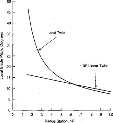
The lift on the entire blade is the integration of the lift on all the blade elements from the center of the rotor to the tip. In order to perform the integration in a tidy manner, the blade will be assumed to have ideal twist. Most helicopter blades are twisted such that the pitch at the tip is less than the pitch at the root. The most common twist is linear such that:

0 — 0O +

where 0O is the pitch that the blade would have if it extended into the center of rotation and 0г is the angle of twist or washout between the center of rotation and the tip. The value of linear twist in current use is from —5° to —16°. For blades with ideal twist instead of linear twist, the local value of pitch is:

A

r/R where 0, is the pitch at the blade tip. Plots of blade pitch for a blade with —10 degrees of linear twist and for a blade with ideal twist are shown in Figure 1.7 for approximately the same rotor lift. It will later be shown that the ideal twist produces better rotor performance than any other type of twist, but that the margin of increased performance over linear twist is relatively small. Actual helicopter blades use linear twist instead of ideal twist because of the ease of manufacture. Because of the ease of analysis, however, ideal twist is assumed in this derivation with the consequences of linear twist shown later.

where AL/Ar is the lift per running foot along the blade and is simply a linear—or triangular—lift distribution with respect to blade station. The total lift on the blade is equal to the area of the triangle:

Thus the lift per blade is:

and the total rotor thrust is the lift per blade times the number of blades, b:

Note the similarity of this equation with the equation for the lift of an airplane wing:

Lw=-V2Saa

2

In the case of the rotor, (p/2)({TR)2 is the dynamic pressure based on tip speed, bcR is the total blade area, a is the slope of the airfoil lift curve, and (0, — ф,)/2 is an effective angle of attack.