Our heavyweight helicopter equal in the world does not have
In Rostov started production of the most load-lifting rotary-wing car The Russian holding «Helicopt[...]

Everything about aircrafts and helicopters. News and events in aviation worldwide. Civil, transportation, military helicopters and airplanes.

Everything about aircrafts and helicopters. News and events in aviation worldwide. Civil, transportation, military helicopters and airplanes.

Everything about aircrafts and helicopters. News and events in aviation worldwide. Civil, transportation, military helicopters and airplanes.

Everything about aircrafts and helicopters. News and events in aviation worldwide. Civil, transportation, military helicopters and airplanes.


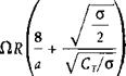
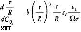
The increment in collective pitch above that required to hover can be estimated from the same principles used for the power increment. The change in pitch can be based on the change in inflow velocity and the tangential flow at the three-quarter radius station.
A A
Д9= .75 (ПК)
For the example helicopter with a vertical rate of climb of 500 ft/min, the additional collective pitch is.4°.
ROTOR THRUST DAMPING
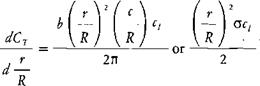
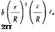
The momentum relationships can be used to derive an approximate equation for the change in rotor thrust coefficient as a result of a change in axial velocity at constant collective pitch. This allows the damping of main rotors and tail rotor to be calculated for use in studies of such maneuvers as jump takeoffs, power failures, and response to pedal inputs.
![]()
A hovering rotor with ideal twist was discussed in Chapter 1. If this rotor is in vertical flight, the equation for CT/a is:
The partial derivative evaluated at the initial value of CT/o is:
![]()
![]()
 |
|
dCT/<5
dVr
This can be used for small rates of descent as well as climb and for inflow through the tail rotor due to turns or sideward flight where the rotor is not in the vortex ring state.
The power required in a vertical climb is higher than that required in hover primarily because of the change in potential energy. Secondary effects are the increased vertical drag, increased tail rotor power, and decreased induced power since the rotor is handling more air. For simple calculations, the profile power of the main and tail rotors can be considered to be the same in climb as in hover.
For this analysis, the equation for vertical drag will be written:
|
^(vlc*VcyAM + (AAzCD) Vc |
|
|
|
|
where AAz is the area of the portion of the airframe not in the wake and CD is the drag coefficient of the additional area.
From the momentum equation:
The tad rotor thrust required to balance main rotor torque is:
Pm Pm
(Щм It
and the tail rotor power is:
R,
(Щм It.
For this analysis, it will be assumed that the tail rotor-induced velocity remains a constant at its hover value and that the tad rotor power is directly proportional to tail rotor thrust alone. The rationale for this assumption is that even though the thrust of the tail rotor increases in climb, it goes into a forward – flight condition where it handles more air and thus produces less induced velocity for the same thrust. The total power is:
and the difference in power between climb and hover is:
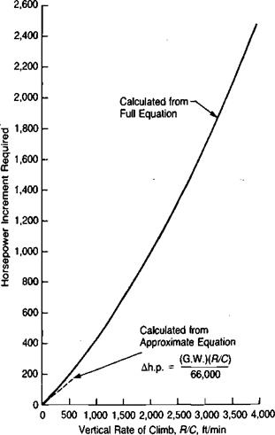
An opportunity to check the validity of this equation is provided by the flight test data of reference 2.1 for an AH-lG. Figure 2.3 shows the correlation and also the difficulty in obtaining this type of test data. For example, at a power increment of 150 h. p., the measured rate of climb varied from 570 to 1,180 ft/min.
Source: Ferrell & Frederickson, “Flight Evaluation Compliance Test Techniques for Army Hot Day Hover Criteria," USAASTA Project 68-55, 1974.
Figure 2.4 presents the results of the same type of analysis for the example helicopter.
A simple method for making a quick estimate of the incremental power for low rates of climb can be obtained by ignoring the vertical drag and tail rotor effects in the above equation. Then:
. G. W. ,
Ah-P – = ^-(4 + Fc-40I)
or
![]()
![]()
![]()
 Ah. p. =
|
It may be seen that for low rates of climb such that
the change in power is simply:
![]() G. W. Vc 550 T
G. W. Vc 550 T
which is just half of the value which would be computed based on the rate of change of potential energy. For the example helicopter at a vertical rate of climb of 500 ft/min—or 8.33 ft/sec—the two velocity terms are:
![]()
and
fa J2 = (39)2 = 1,521
Thus the criterion can be considered to be satisfied for this case. The first approximation to the extra power required to climb at this rate for the example helicopter is 150 h. p., as shown in Figure 2.4. A more detailed analysis of vertical climb is given in reference 2.2.
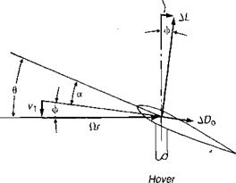
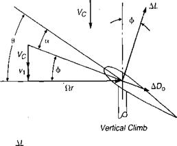
The conditions at the blade element for hover, climb, and descent are shown in Figure 2.2. In climb, the rearward tilt of the lift vector produces extra inflow drag, which is represented by extra power required to climb. In a steady climb, the helicopter is not being accelerated, so the rotor thrust has the same value as in
|
|
|
hover except for minor increases due to the increased vertical drag of the fuselage. This means that the average angle of attack is essentially the same as in hover; but, because of the extra inflow through the rotor, the blade pitch must be increased over the hover value. For calculations of the vertical climb, the combined momentum and blade element method developed for the hover analysis can be modified to include the effect of climb by using the general equation for induced velocity:
8л
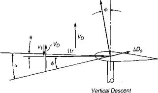
In descent, the blade element is subjected to air coming up at it from below. This reduces the rearward tilt of the thrust vector, thus reducing the power required. The upward velocity also means that the blade pitch must be reduced to hold the average angle of attack and the same rotor thrust.
At some rate of descent, the forward tilt of the lift vector is equal to the drag component. This is the condition of autorotation, since no torque need be
applied to maintain rotor speed. In an actual rotor, some blade elements will have more drag than the forward component of lift; but on other elements the situation will be reversed. Autorotation occurs when the integration of torque along the blade is zero—or, for an actual helicopter, is sufficiently negative to make up for losses in the tail rotor, transmissions, and accessories. All helicopters are equipped with an overrunning clutch between the transmission and the engine, so that the rotor does not have to drive a dead engine in autorotation.
Vertical autorotation is a balanced, steady flight condition in which the rotor thrust is equal to the gross weight and the rotor speed remains constant. For a given helicopter at a given gross weight, there is a unique combination of rate of descent, rotor speed, and blade pitch that defines the condition. Autorotation, once established, is stable: if the rotor speed decreases, the horizontal velocity vector at the blade element, Ctr, will shorten, and the lift vector will be tilted further forward, thus tending to increase rotor speed. The opposite effect occurs if the rotor speed increases from its original value. The pilot can control rotor speed by adjusting the blade pitch. A reduction of pitch initially decreases the rotor lift so that the rate of descent increases, thus tilting the lift vector forward and accelerating the rotor. As the rotor speeds up, the lift again reaches a value equal to the weight of the helicopter, and a new set of equilibrium conditions is reached with a higher rotor speed and a slightly different rate of descent than before the blade pitch was decreased.
For each helicopter, there is an upper and a lower limit of rotor speed that the pilot must observe. The upper limit is the speed at which the centrifugal forces in the blades and hub reach the structural design limit. The lower limit is the speed at which, in order to maintain rotor thrust equal to the gross weight, each blade element is being operated at or near its stall angle of attack. Once the blade elements stall, the drag increases rapidly, as shown in Figure 1.10 of Chapter 1, and becomes greater than any forward tilt of the lift vector can compensate. At this point the rotor slows down to a stop, and the flight becomes an accident. The upper limit is generally 10-20% above the normal speed for hover, and the lower limit may be as low as 20-30% below the normal speed.
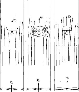
The tunnel fan induces an upward velocity of about the same magnitude as the rotor-induced velocity. The rotor operates in a doughnut-shaped mass of revolving air, which goes down through the rotor and up around the outside of the tips. This is the vortex ring state. Since no definite and continuous wake exists, the momentum concepts cannot be used. In the extreme case, when the rate of descent is equal to the induced velocity, there is no net mass flow through the rotor, and the momentum equations would indicate that no thrust could be developed. In reality, however, the rotor does have a significant thrust capability even in this condition. The classical boundaries of the vortex ring state are from hover to a rate of descent equal to twice the hover-induced velocity.
Windmill Brake State
If the tunnel upflow is increased to the point where it is higher than the rotor – induced velocity, both the local flow at the rotor and the flow in the remote field are up; there is a well-behaved wake above the rotor, and the momentum concepts can again be used. This condition is known as the windmill brake state, and its governing equation is:
STATES OF FLOW
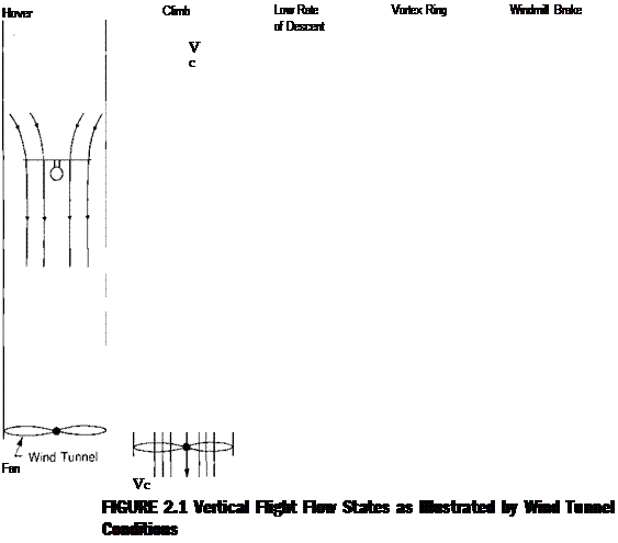
Just as in hover, there are two ways to analyze the rotor in vertical flight, the momentum method and the blade element method. In some vertical flight conditions, however, the relationships do not exist that were used to develop the hover methods. To obtain a physical understanding of the problem, let us examine the flow around a rotor mounted in an open-ended vertical wind tunnel as in Figure 2.1. Several different types of flight conditions can be simulated:
Hover
The tunnel fan is stopped and the rotor produces flow down through the tunnel. The governing momentum equation is:
|
|
Climb
The tunnel fan is used to induce a downflow in addition to that of the rotor. Both the local flow at the rotor and the remote flow are down. The induced velocity at the rotor is:
 |
|
|
|
|
|
![]()
![]()
![]()
 |
or assuming constant thrust conditions:
where Vc is the climb velocity in feet per second.
Low Rate of Descent
The tunnel fan is used to induce a small upflow in the tunnel. For this case the flow is mixed. The local flow near the rotor is dominated by the rotor-induced velocity and is down, but the rest of the flow Field is up.
 |
From a momentum standpoint, the equation for the induced velocity is:
This equation is semivalid for very low rates of descent; but, because of the mixed conditions, the continuous-flow assumption on which the momentum theory is based breaks down when the rate of descent is approximately a quarter of the hover-induced velocity.
The following items can be evaluated by the methods in this chapter.
page
Coefficients, nondimensional 15
Coning 31
Contraction of wake, effect on power 58
Disc loading, effective 35
Download penalty 7
Drag coefficient, average 24
Drag divergence penalty 63
Figure of Merit 26
Ground effect 67
Hover performance, numerical calculation method 69
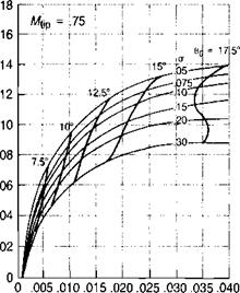
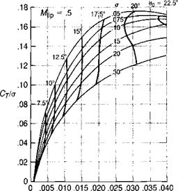
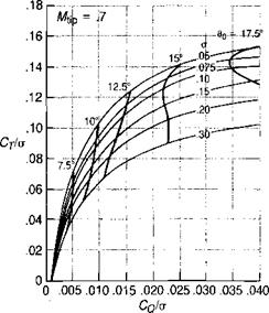
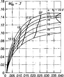
Hover performance, chart method 81
Induced velocity in wake 4
Induced velocity distribution 38
Lift coefficient, average 18
Lock number 31
Pitch at tip, ideal 19
Power coefficient, ideal twist 22
Power, induced 8
Power loading 9
Rotation of wake, effect on induced power 52
Rotational velocity 54
Solidity 16
Stall penalty 63
Tip loss 34
Tip speed from rpm 11
Twist, effect on power 41
|
|
|
|
|
|
|
|
|
|
|
 |
|
|
|
|
|
|
|
|
|
|
|
|
 |
|
|
|
|
 |
|
|
page |
|
|
Disc loading |
5 |
|
Induced velocities in wake |
5 |
|
Vertical drag |
7 |
|
Power loading |
9 |
|
Power to hover, main rotor |
9 |
|
Solidity |
16 |
|
CjIg |
18 |
|
Average lift coefficient |
18 |
|
Tip angle |
19 |
|
Collective pitch |
20 |
|
Average drag coefficient |
24 |
|
Lock number |
31 |
|
Coning in hover |
32 |
|
Main rotor tip loss factor |
34 |
|
Effective disc loading |
35 |
|
Effective induced velocity |
35 |
|
Tip angle with tip and root losses |
36 |
|
Hover power with tip and root losses |
36 |
|
Blade element conditions |
41 |
|
Effect of twist |
42 |
|
Power due to wake rotation |
52 |
|
Ground effect |
68 |
|
Main rotor hover power |
75 |
|
Tail rotor hover power |
75 |
|
Blade element conditions |
76 |
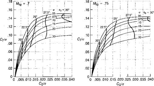
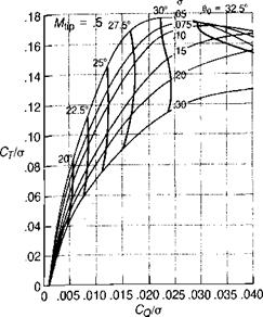
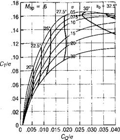
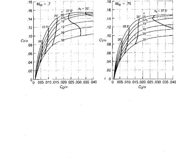
The hover performance of a new rotor design may be estimated using test data from a previously tested rotor, even if they are not identical. The effect of differences in solidity, twist, number of blades, and tip Mach number can be estimated from the hover charts and used as correction factors.
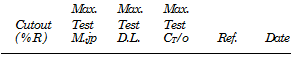
Table 1.1 lists a number of whirl tower tests and the characteristics of the rotors tested.
![]()
|
19 18 17 16 15 14 13 12 11 10 9 8 7 6 5 4 З 2 1 0 |
|
|
||
|
|||
|
|||
|
|||
|
|||
|
|||
|
![]()

|
TABLE 1.1 Tabulation of Published Whirl Tower Tests Chord
|
 Airfoil
|
0015 |
14 |
.22 |
3 |
.117 |
1.26 |
1937 |
|
23015 |
12 |
.69 |
6.6 |
.177 |
1.27 |
1952 |
|
23015 |
12 |
.69 |
5.7 |
.164 |
1.27 |
1952 |
|
8H12 |
10 |
.58 |
5.9 |
.146 |
1.28 |
1954 |
|
63 2—015 |
15 |
.71 |
6.1 |
.192 |
1.29 |
1956 |
|
0012 |
20 |
.45 |
2.5 |
.066 |
1.30 |
1956 |
|
0017 to 0009 |
14 |
.72 |
4.9 |
.158 |
1.31 |
1958 |
|
0015 |
14 |
.81 |
4.7 |
.189 |
1.32 |
1958 |
|
0012 |
15 |
.70 |
4.4 |
.191 |
1.1 |
1958 |
|
0012 |
18 |
.98 |
22 |
.118 |
1.33 |
1960 |
|
63215A018 |
14 |
.76 |
7.0 |
.177 |
1.34 |
1960 |
|
0012 |
25 |
.95 |
14 |
.136 |
1.35 |
1961 |
|
632A015(230) |
14 |
, .67 |
3.8 |
.195 |
1.8 |
1961 |
|
632A012(130) |
15 |
.75 |
5.1 |
.179 |
1.36 |
1962 |
|
0012 |
10 to 50 |
.67 |
13.7 |
.108 |
1.37 |
1970 |
|
13006 |
10 |
.58 |
33 |
.111 |
1.24 |
1971 |
|
TABLE 1.1 (continued)
|
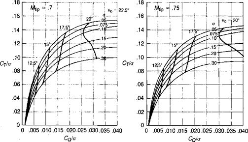
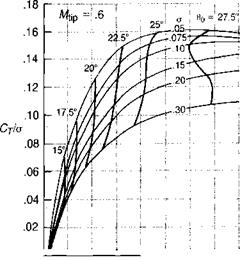
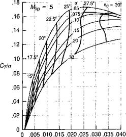
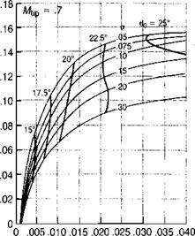
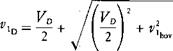
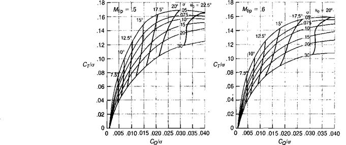
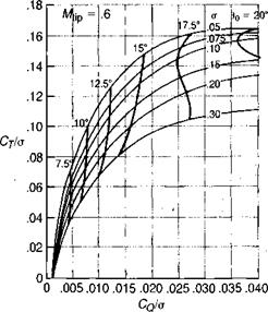
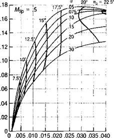
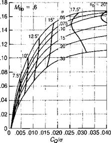
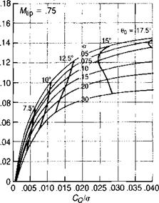
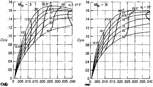
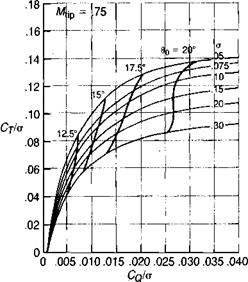
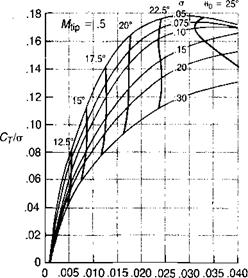
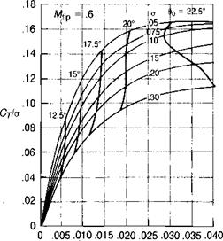
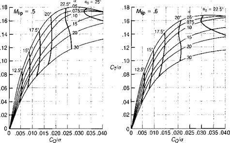
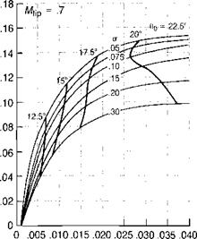
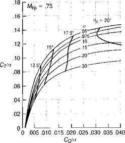
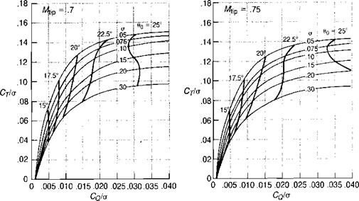
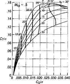
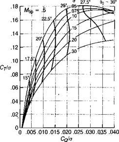
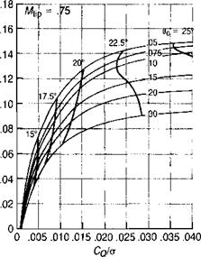
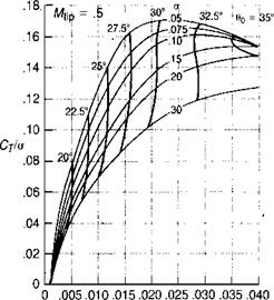
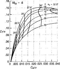
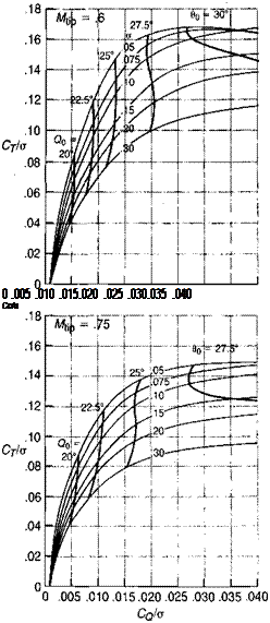
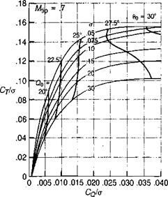
The hover charts starting on page 81 were prepared using the combined momentum and blade element method just described. The charts are based on the following assumptions: [2]
|
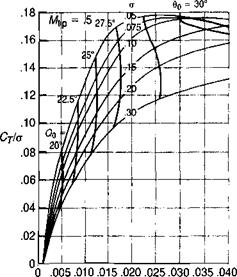
CqIg FIGURE 1.44 Calculated Performance of Isolated Main and Tail Rotors of Example Helicopter |
• NACA 0012 airfoil characteristics based on the whirl tower tests of reference 1.1. Thus the Reynolds number characteristics correspond to a 16-inch chord.
• Blade cutout = 0.15 R
1. Given: Rotor geometry—number of blades, radius, chord, twist, cutout, airfoil data; and test conditions—tip speed, atmospheric density, speed of sound.
2. Select a finite number of blade elements (at least five but not more than fifteen).
3. At the boundary between each blade element, tabulate: nondimen – sional blade station r/R nondimensional chord, c/R local Mach number, M — (f/RJKnRJ/FsJ; slope of lift curve, a =/(M), per radian, from airfoil data such as Figure 1.10; local twist, A0.
4. Choose collective pitch, 90; tabulate pitch at boundary between each blade element:
9 = 90 + Л9 – aL0
Note: Choose minimum value of 0O so that 0 is always positive.
5. Calculate the local inflow angle
![]()
|
|
|
|
|
|
|
|

![]()
 |
||||
or, for a constant chord blade:
Note: 0 and a are in radian units in this equation.
6. Calculate the local angle of attack:
A
a = 0 — tan-1 — degrees
л Ы
7. Using curves of airfoil data such as Figure 1.10 or equations such as those developed in Chapter 6, tabulate ct and cd for the local angle of attack and Mach number. Note: If airfoil data synthesized from whirl tower or model rig test results are being used, they already include the compressibility tip relief effect. If, on the other hand, airfoil data from a two-dimensional wind tunnel are being used, the tip relief may be accounted for by reducing the local Mach number of the outer 10% of the blade by the increment corresponding to the thickness ratio of the tip airfoil from Figure 3.38 of Chapter 3.
8.
 |
Compute the running thrust loading:
9.
 |
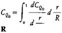
Integrate either graphically or numerically to obtain the thrust coefficient without tip loss:
10. Calculate tip loss factor:
![]() B= 1
B= 1
Note: All the airfoil data tabulated in Chapter 6 as originating from whirl tower or model rig test results were synthesized from two-bladed
rotors with the assumption that the effective radius was constant at
0. 97 R. If these airfoil data are used, the same assumption should be made, at least in the range of thrust coefficients used in the tests. A study using the airfoil data from reference 1.1 indicates that satisfactory correlation is obtained for a wide range of rotor parameters if the following effective radius equations are used:

for Cr < 0.006
11.
 |
Calculate the corrected thrust coefficient using either graphical or numerical integration:
12.
 |
Compute the running profile torque loading:
13.
 |
Integrate for the profile torque coefficient:
14.
 |
Compute the running induced torque loading:
15.
 |
Integrate for the induced torque coefficient:
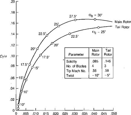
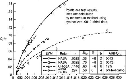
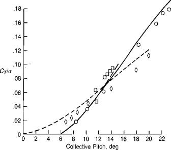
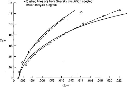
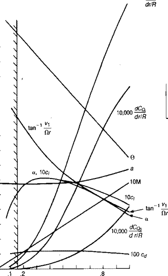
The method has been used with the synthesized 0012 airfoil characteristics on several rotors for which whirl tower data have been published. Figure 1.42 shows correlation with the NACA two-bladed, low-solidity rotor of reference 1.1; the moderate solidity CH-53A rotor of reference 1.5; and the high solidity AH – 56A tail rotor of reference 1.24. It may be seen that the correlation is satisfactory both in power and in collective pitch. Figure 1.43 presents test results from two Sikorsky whirl tower tests, one for a main rotor and the other for a tail rotor. The test points are compared with the results of two calculation schemes: the momentum-blade element method of this book; and the Circulation Coupled Hover Analysis Program (CCHAP) described in reference 1.25. It may be seen that the momentum-blade element method gives satisfactory correlation except at very high thrust levels and is therefore adequate for most hover calculations of a practical, engineering nature. Figure 1.44 shows the performance of the main and tail rotors of the example helicopter calculated by the simple method, and
|
CqI(j |
|
FIGURE 1.42 Correlation of Test Results with Calculated Results |
Source: Carpenter, “Lift and Profile-Drag Characteristics of a NACA 0012 Airfoil Section as Derived from Measured Helicopter-Rotor Hovering Performance,” NACA TN 4357, 1958; Landgrebe, “An Analytical and Experimental Investigation of Helicopter Rotor Hover Performance and Wake Geometry Characteristics," USAAMRDLTR 71-24, 1971; Johnston & Cook, "AH-56A Vehicle Development,” AHS 27th Forum, 1971.
|
Symb. |
Rotor |
a |
Mtip |
©1 |
b |
Airfoil |
Ref. |
|
0 |
"Baseline" main rotor |
.0894 |
.523 |
-9.25 |
6 |
0012 |
1.40 |
|
A |
Tail rotor |
.20 |
.63 |
-8 |
4 |
0012 |
1:24 |
|
• Points are test results. • Solid lines are from momentum method of this book. |
|
FIGURE 1.43 Correlation of Prediction Methods with Sikorsky Whirl Tower Test Data |
Source: Rorke, "Hover Performance Tests of Full Scale Variable Geometry Rotors,” NASA CR 2713, 1976; Landgrebe, “Aerodynamic Theory for Advanced Rotorcraft” JAHS 22-2, 1977.
Figure 1.45 shows the various elements of the calculation for the main rotor at a collective pitch of 17.5°.